Processes and model formulation
Domain and definitions
Coordinate system
XBeach uses a coordinate system where the computational x-axis is always oriented towards the coast, approximately perpendicular to the coastline, and the y-axis is alongshore, see Fig. 1 and Fig. 2. This coordinate system is defined in world coordinates. The grid size in x- and y-direction may be variable but the grid must be curvilinear. Alternatively, in case of a rectangular grid (a special case of a curvilinear grid) the user can provide coordinates in a local coordinate system that is oriented with respect to world coordinates (xw, yw) through an origin (xori, yori) and an orientation (alfa) as depicted in Fig. 1. The orientation is defined counter-clockwise w.r.t. the xw-axis (East).
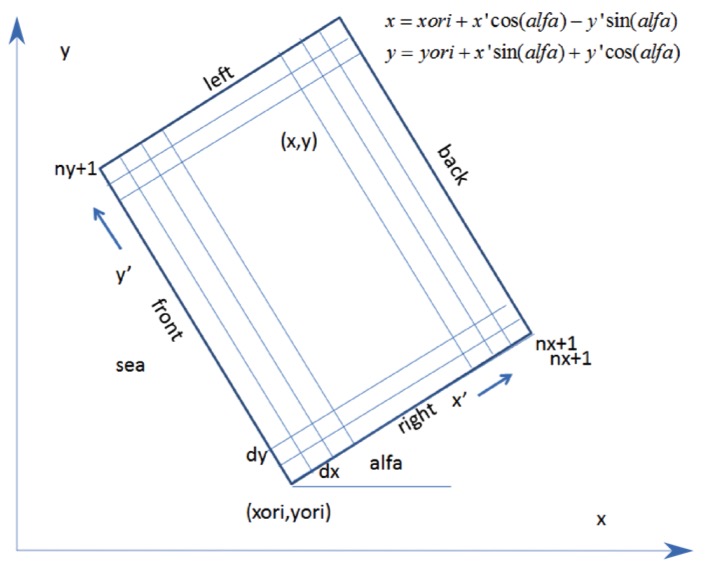
Fig. 1 Rectangular coordinate system of XBeach
Grid set-up
The grid applied is a staggered grid, where the bed levels, water levels, water depths and concentrations are defined in cell centers, and velocities and sediment transports are defined in u- and v-points, viz. at the cell interfaces. In the wave energy balance, the energy, roller energy and radiation stress are defined at the cell centers, whereas the radiation stress gradients are defined at u- and v-points.
Velocities at the u- and v-points are denoted by the output variables uu and vv respectively; velocities u and v at the cell centers are obtained by interpolation and are for output purpose only. The water level, zs, and the bed level, zb, are both defined positive upward. uv and vu are the u-velocity at the v-grid point and the v-velocity at the u-grid point respectively. These are obtained by interpolation of the values of the velocities at the four surrounding grid points.
The model solves coupled 2D horizontal equations for wave propagation, flow, sediment transport and bottom changes, for varying (spectral) wave and flow boundary conditions.
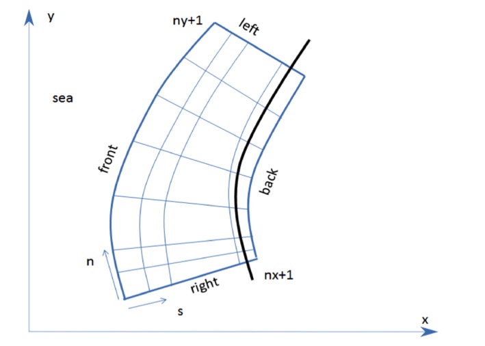
Fig. 2 Curvilinear coordinate system of XBeach
Hydrodynamics options
XBeach was originally developed as a short-wave averaged but wave-group resolving model, allowing resolving the short wave variations on the wave group scale and the long waves associated with them. Since the original paper by Roelvink et al. [2009] a number of additional model options have been implemented, thereby allowing users to choose which time-scales to resolve:
Stationary wave model (keyword: wavemodel = stationary), efficiently solving wave-averaged equations but neglecting infragravity waves;
Surfbeat mode (instationary) (keyword: wavemodel = surfbeat), where the short wave variations on the wave group scale (short wave envelope) and the long waves associated with them are resolved;
Non-hydrostatic mode (wave-resolving) (keyword: wavemodel = nonh), where a combination of the non-linear shallow water equations with a pressure correction term is applied, allowing to model the propagation and decay of individual waves.
In the following these options are discussed in more detail. Important to note that all times in XBeach are prescribed on input in morphological time. If you apply a morphological acceleration factor (keyword: morfac) all input time series and other time parameters are divided internally by morfac. This way, you can specify the time series as real times, and vary the morfac without changing the rest of the input files (keyword: morfacopt = 1).
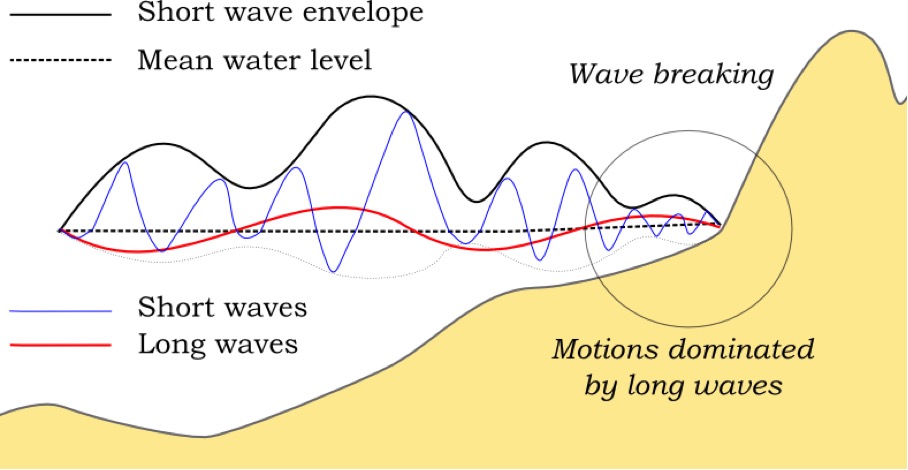
Fig. 3 Principle sketch of the relevant wave processes
Stationary mode
See also
The stationary mode is implemented in mod:wave_stationary_module.
In stationary mode the wave-group variations and thereby all infragravity motions are neglected. This is useful for conditions where the incident waves are relatively small and/or short, and these motions would be small anyway. The model equations are similar to HISWA ([Holthuijsen et al., 1989]) but do not include wave growth or wave period variations. Processes that are resolved are wave propagation, directional spreading, shoaling, refraction, bottom dissipation and wave breaking, and a roller model is included; these processes are usually dominant in nearshore areas of limited extent. For the breaking dissipation we use the Baldock et al. [1998] model, which is valid for wave-averaged modeling. The radiation stress gradients from the wave and roller model force the shallow water equations, drive currents and lead to wave setdown and setup. Additionally, wind and tidal forcing can be applied.
The mean return flow due to mass flux and roller is included in the model and affects the sediment transport, leading to an offshore contribution. To balance this, effects of wave asymmetry and skewness are included as well. Bed slope effects can further modify the cross-shore behavior. A limited number of model coefficients allow the user to calibrate the profile shape resulting from these interactions.
A typical application would be to model morphological changes during moderate wave conditions, often in combination with tides. The wave boundary conditions can be specified as constant (keyword: wbctype = params) or as a time-series of wave conditions (keyword: wbctype = jonstable). Typical examples of such model applications are given below for tombolo formation behind an offshore breakwater (left panel) and development of an ebb delta at a tidal inlet (right panel). A big advantage of the stationary XBeach wave model over other models is that the lateral boundaries are entirely without disturbance if the coast is longshore uniform near these boundaries.
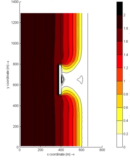
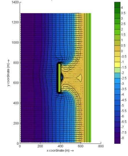
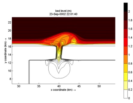
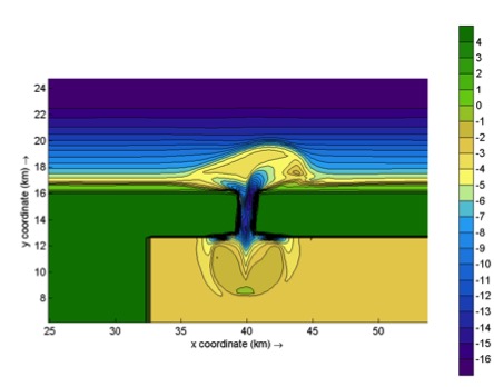
Root-mean square wave height (left panels) and final bathymetry (right panels) for an offshore breakwater case (upper panels) and a tidal inlet with waves from 330 degrees (lower panels).
Surf beat mode (instationary)
See also
The surfbeat mode is implemented in mod:wave_instationary_module.
The short-wave motion is solved using the wave action equation which is a time-dependent forcing of the HISWA equations [Holthuijsen et al., 1989]. This equation solves the variation of short-waves envelope (wave height) on the scale of wave groups. It employs a dissipation model for use with wave groups [Daly et al., 2012, Roelvink, 1993] and a roller model [Nairn et al., 1990, Stive and De Vriend, 1994, Svendsen, 1984] to represent momentum stored at the surface after breaking. These variations, through radiation stress gradients [Longuet-Higgins and Stewart, 1962, Longuet-Higgins and Stewart, 1964] exert a force on the water column and drive longer period waves (infragravity waves) and unsteady currents, which are solved by the nonlinear shallow water equations [Phillips, 1977]. Thus, wave-driven currents (longshore current, rip currents and undertow), and wind-driven currents (stationary and uniform) for local wind set-up, long (infragravity) waves, and runup and rundown of long waves (swash) are included.
Using the surfbeat mode is necessary when the focus is on swash zone processes rather than time-averaged currents and setup. It is fully valid on dissipative beaches, where the short waves are mostly dissipated by the time they are near the shoreline. On intermediate beaches and during extreme events the swash motions are still predominantly in the infragravity band and so is the runup.
Under this surfbeat mode, several options are available, depending on the circumstances:
1D cross-shore; in this case the longshore gradients are ignored and the domain reduces to a single gridline (keyword: ny = 0). Within this mode the following options are available:
Retaining directional spreading (keyword: dtheta < thetamax - thetamin); this has a limited effect on the wave heights because of refraction, but can also allow obliquely incident waves and the resulting longshore currents;
Using a single directional bin (keyword: dtheta = thetamax- thetamin); this leads to perpendicular waves always and ignores refraction. If the keyword snells = 1 is applied, the mean wave direction is determined based on Snells law. In this case also longshore currents are generated.
2DH area; the model is solved on a curvilinear staggered grid (rectilinear is a special case). The incoming short wave energy will vary along the seaward boundary and in time, depending on the wave boundary conditions. This variation is propagated into the model domain. Within this mode the following options are available:
Resolving the wave refraction ‘on the fly’ using the propagation in wave directional space. For large directional spreading or long distances this can lead to some smoothing of groupiness since the waves from different directions do not interfere but their energy is summed up. This option is possible for arbitrary bathymetry and any wave direction. The user must specify the width of the directional bins for the surfbeat mode (keyword: dtheta)
Solving the wave direction at regular intervals using the stationary solver, and then propagating the wave energy along the mean wave direction. This preserves the groupiness of the waves therefore leads to more forcing of the infragravity waves (keyword: single_dir = 1). The user must now specify a single directional bin for the instationary mode (dtheta = thetamax - thetamin) and a smaller bin size for the stationary solver (keyword: dtheta_s).
For schematic, longshore uniform cases the mean wave direction can also be computed using Snells law (keyword: snells = 1). This will then give comparable results to the single_dir option.
In the figures below some typical applications of 1D and 2D models are shown; a reproduction of a large-scale flume test, showing the ability of XBeach to model both short-wave (HF) and long-wave (LF) wave heights and velocities; and a recent 2DH simulation [Nederhoff et al., 2015] of the impact of hurricane Sandy on Camp Osborne, Brick, NJ.
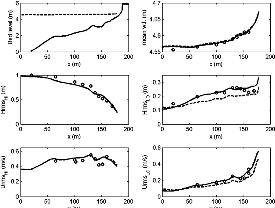
Fig. 4 Computed and observed hydrodynamic parameters for test 2E of the LIP11D experiment. Top left: bed level and mean water level. Top right: measured (dots) and computed as simulated by XBeach
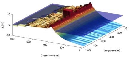
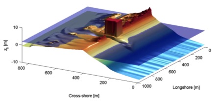
Pre (left) and post-Sandy (right) in a three dimensional plot with both bed and water levels as simulated by XBeach ([Nederhoff et al., 2015])
Non-hydrostatic mode (wave resolving)
See also
The non-hydrostatic mode is implemented in mod:nonh_module.
For non-hydrostatic XBeach calculations (keyword: wavemodel = nonh) depth-averaged flow due to waves and currents are computed using the non-linear shallow water equations, including a non-hydrostatic pressure. The depth-averaged normalized dynamic pressure (\(q\)) is derived in a method similar to a one-layer version of the SWASH model [Zijlema et al., 2011]. The depth averaged dynamic pressure is computed from the mean of the dynamic pressure at the surface and at the bed by assuming the dynamic pressure at the surface to be zero and a linear change over depth.
Under these formulations dispersive behavior is added to the long wave equations and the model can be used as a short-wave resolving model. Wave breaking is implemented by disabling the non-hydrostatic pressure term when waves exceed a certain steepness, after which the bore-like breaking implicit in the momentum-conserving shallow water equations takes over.
In case the non-hydrostatic mode is used, the short wave action balance is no longer required. This saves computation time. However, in the wave-resolving mode we need much higher spatial resolution and associated smaller time steps, making this mode much more computationally expensive than the surfbeat mode.
The main advantages of the non-hydrostatic mode are that the incident-band (short wave) runup and overwashing are included, which is especially important on steep slopes such as gravel beaches. Another advantage is that the wave asymmetry and skewness are resolved by the model and no approximate local model or empirical formulation is required for these terms. Finally, in cases where diffraction is a dominant process, wave-resolving modeling is needed as it is neglected in the short wave averaged mode. The XBeach-G formulations for gravel beaches [McCall et al., 2014] are based on the non-hydrostatic mode. Although sandy morphology can be simulated using the wave-resolving mode, it has not been extensively validated and it is likely that changes in the sediment transport formulations will be implemented in the near future.
To improve the dispersive behaviour a (reduced) 2-layer non-hydrostatic is implemented as well [de Ridder et al., 2021]. In this version (keyword: nhq3d = 1, see Section Reduced two layer model (nh+)), the pressure in the vertical is described by a hydrostatic pressure assumption in the bottom layer, and a non-hydrostatic distribution in the upper layer.
An interesting recent application that has been validated for a number of cases concerns the modeling of primary waves generated by large ships, see Ship-induced wave motions.

Fig. 5 Measured (black) and modeled (red) time series of overtopping during BARDEX experiment, from [McCall et al., 2014].
Short wave action
Short wave action balance
See also
The short wave action balance is implemented in func:wave_instationary_module/wave_instationary.
The wave forcing in the shallow water momentum equation is obtained from a time dependent version of the wave action balance equation. Similar to Delft University (stationary) HISWA model ([Holthuijsen et al., 1989]) the directional distribution of the action density is taken into account, whereas the frequency spectrum is represented by a frequency, best represented by the spectral parameter \({f}_{m-1,0}\). The wave action balance (keyword: swave) is then given by:
In which the wave action \(A\) is calculated as:
where \(\theta\) represents the angle of incidence with respect to the x-axis, \({S}_{w}\) represents the wave energy density in each directional bin and \(\sigma\) the intrinsic wave frequency. The intrinsic frequency \(\sigma\) and group velocity \({c}_{g}\) is obtained from the linear dispersion relation. The intrinsic frequency is for example obtained with:
The wave action propagation speeds in \(x\), \(y\) and directional space are given by:
where \(h\) represents the local water depth and \(k\) the wave number. The intrinsic wave frequency \(\sigma\) is determined without wave current interaction (keyword: wci = 1, see Section 2.3.1.1), which means it is equal to the absolute radial frequency \(\omega\).
Wave-current interaction (wci)
See also
The wave-current interaction is implemented in func:wave_instationary_module/wave_instationary.
Wave-current interaction is the interaction between waves and the mean flow. The interaction implies an exchange of energy, so after the start of the interaction both the waves and the mean flow are affected by each other. This feature is especially of importance in gullies and rip-currents ([Reniers et al., 2007]).
In XBeach this is taken into account by correcting the wave number \(k\) with the use of Eikonal equations, which will have impact on the group and wave propagation speed (x, y, and directional space). The cross-shore and alongshore wave numbers, \({k}_{x}\) and \({k}_{y}\), are defined according to equation (5). In these formulations the subscripts refer to the direction of the wave vector components.
Where subscript \(n-1\) refers the wave number of the previous time step, \(k_{x}^{:}\) and \(k_{y}^{:}\) are the wave number corrections and \({k}_{x}\) and \({k}_{y}\) are the corrected wave numbers that take into account the presence of a current. The correction terms are determined with a second set of equations, the Eikonal equations:
The wave number is then given by:
The absolute radial frequency \(\omega\) is calculated with:
where \({u}^{L}\) and \({v}^{L}\) are the cross-shore and alongshore depth-averaged Lagrangian velocities respectively. The wave action propagation speed (in x and y direction) is given by:
The propagation speed in directional (\(\theta\)) space, where bottom refraction (first term) and current refraction (last two terms) are taken into account, is obtained from:
Dissipation
In XBeach there are three short wave dissipation processes that can be accounted for: wave breaking (\({D}_{w}\)), bottom friction (\({D}_{f}\)) and vegetation (\({D}_{v}\)). The three processes are explained in more detail in the following subsections.
Wave breaking
See also
Short wave dissipation by breaking is implemented in mod:roelvink_module.
Five different wave breaking formulations are implemented in XBeach. The formulations can be selected using the keyword break (Table 1).
Wave breaking formula |
Type of waves |
keyword |
|---|---|---|
Roelvink (1993a) |
Instationary |
roelvink1 |
Roelvink (1993a) extended |
Instationary |
roelvink2 |
Daly et al. (2010) |
Instationary |
roelvink_daly |
Baldock et al. (1998) |
Stationary |
baldock |
Janssen & Battjes (2007) |
Stationary |
janssen |
For the surf beat approach the total wave energy dissipation, i.e. directionally integrated, due to wave breaking can be modeled according to [Roelvink, 1993] (keyword: break = roelvink1). In the formulation of the dissipation due to wave breaking the idea is to calculate the dissipation with a fraction of breaking waves (\({Q}_{b}\)) multiplied by the dissipation per breaking event. In this formulation \(\alpha\) is applied as wave dissipation coefficient of O (keyword: alpha), \({T}_{rep}\) is the representative wave period and \({E}_{w}\) is the energy of the wave. The fraction of wave breaking is determined with the root-mean-square wave height (\({H}_{rms}\)) and the maximum wave height (\({H}_{max}\)). The maximum wave height is calculated as ratio of the water depth (\(h\)) plus a fraction of the wave height (\(\delta H_{rms}\), keyword: delta) using a breaker index \(\gamma\) (keyword: gamma). In the formulation for \({H}_{rms}\) the \(\rho\) represents the water density and \(g\) the gravitational constant. The total wave energy \({E}_{w}\) is calculated by integrating over the wave directional bins.
In variation of (11), one could also use another wave breaking formulation, presented in (12). This formulation is somewhat different than the formulation of [Roelvink, 1993] and selected using keyword break = roelvink2. The main difference with the original formulation is that wave dissipation with break = roelvink2 is proportional to \({H}^{3} / h\) instead of \({H}^{2}\).
Alternatively the formulation of [Daly et al., 2010] states that waves are fully breaking if the wave height exceeds a threshold (\(\gamma\)) and stop breaking if the wave height fall below another threshold (\(\gamma_{2}\)). This formulation is selected by break = roelvink_daly and the second threshold, \(\gamma_{2}\), can be set using keyword gamma2.
In case of stationary waves [Baldock et al., 1998] is applied (keyword: break = baldock), which is presented in (14). In this breaking formulation the fraction breaking waves \({Q}_{b}\) and breaking wave height \({H}_{b}\) are calculated differently compared to the breaking formulations used for the non-stationary situation. In \(\alpha\) is applied as wave dissipation coefficient, \({f}_{rep}\) represents a representative intrinsic frequency and \(y\) is a calibration factor.
Finally, it is possible to use the [Janssen and Battjes, 2007] formulation for wave breaking of stationary waves (keyword: break = janssen). This formulation is a revision of Baldock’s formulation.
In both the instationary or stationary case the total wave dissipation is distributed proportionally over the wave directions with the formulation in (16).
Bottom friction
See also
Short wave dissipation by bottom friction is implemented in func:wave_instationary_module/wave_instationary.
The short wave dissipation by bottom friction is modeled as
In (17) the \({f}_{w}\) is the short-wave friction coefficient. This value only affects the wave action equation and is unrelated to bed friction in the flow equation. Studies conducted on reefs (e.g. [Lowe et al., 2007]) indicate that \({f}_{w}\) should be an order of magnitude (or more) larger than the friction coefficient for flow (\({c}_{f}\)) due to the dependency of wave frictional dissipation rates on the frequency of the motion.
The derivation of the short wave dissipation term is based time-averaged instantaneous bottom dissipation using the Johnson friction factor \({f}_{w}\) of the bed shear stress:
The evaluation of the term \(\left\langle\left|\tilde{u}\right|^{3}\right\rangle\), the so-called third even velocity moment, depends on the situation. First we need expressions for the orbital velocity amplitude, which is expressed as:
In this formulation \({T}_{p}\) is the peak wave period, \({H}_{rms}\) is the root-mean-square wave height, \(k\) is the wave number and \(h\) is the local water depth.
If we consider the slowly-varying dissipation in wave groups, we need only to average over a single wave period and we can use a monochromatic (regular wave) expression. If we want to have the time-average dissipation over a full spectrum we get the best approximation from considering a linear Gaussian distribution. [Guza and Thornton, 1985] give pragmatic expressions for both cases.
For the monochromatic case:
For the linear Gaussian approximation:
Combining (18) and (20) we get:
In XBeach the orbital velocity amplitude is computed as in
orbital-velocity-monochromatic and the dissipation according to
(22), which is correct for the case
of instationary simulations on wave-group scale.
For the stationary case formulations (18) and (21) are similarly combined into:
Vegetation
See also
Short wave dissipation by vegetation is implemented in mod:vegetation_module.
The presence of aquatic vegetation within the area of wave propagation or wave breaking results in an additional dissipation mechanism for short waves. This is modeled using the approach of [Mendez and Losada, 2004], which was adjusted by [Suzuki et al., 2012] to take into account vertically heterogeneous vegetation, see [van Rooijen et al., 2015]. The short wave dissipation due to vegetation is calculated as function of the local wave height and several vegetation parameters. The vegetation can be schematized in a number of vertical elements with each specific property. In this way the wave damping effect of vegetation such as mangrove trees, with a relatively dense root system but sparse stem area, can be modeled. The dissipation term is then computed as the sum of the dissipation per vegetation layer ([Suzuki et al., 2012]):
where \({D}_{v,i}\) is the dissipation by vegetation in vegetation layer \(i\) and \({n}_{v}\) is the number of vegetation layers. The dissipation per layer is given by:
where \(\widetilde{C}_{D,i}\) is a (bulk) drag coefficient, \({b}_{v,i}\) is the vegetation stem diameter, \({N}_{v,i}\) is the vegetation density, and \(\alpha_{i}\) is the relative vegetation height (= \({h}_{v} / h\)) for layer \(i\). In case only one vegetation layer is specified, the plants are assumed to be vertically uniform, which would for example typically apply in case of modeling sea grass.
Radiation stresses
Given the spatial distribution of the wave action (and therefore wave energy) the radiation stresses can be evaluated by using linear wave theory as described by:
Wave shape
See also
Wave shapes are implemented in func:morphevolution/RvR and func:morphevolution/vT.
The morphodynamic model considered is (short) wave averaged and resolves hydrodynamics associated with the wave group time scale. As a result the short wave shape is not solved for. However, as waves propagate from deep water onto beaches, their surface form and orbital water motion become increasingly non-linear because of the amplification of the higher harmonics.
There are two wave forms implemented to take this non-linearity into account:
A formulation of [Ruessink et al., 2012] based on a parameterization with the Ursell number. (keyword: waveform = ruessink_vanrijn)
A formulation of [van Thiel de Vries, 2009] based on the parameterized wave shape model of [Rienecker and Fenton, 1981] (keyword: waveform = vanthiel)
The formulation of [Ruessink et al., 2012] relies on parameterizations for the non-linearity parameter \(r\) and phase \(\Phi\). The parameterizations are based on a data set of 30.000+ field observations of the orbital skewness \({S}_{k}\) and asymmetry \({A}_{s}\), collected under non-breaking and breaking wave conditions. The only variable parameter is the Ursell number, since according to [Ruessink et al., 2012] the Ursell that includes \({H}_{s}\), \(T\) and \(h\), describes the variability in \({S}_{k}\) and \({A}_{s}\) well. The Ursell number is calculated with the equation below.
The value for the skewness and asymmetry is calculated with the use of a Boltzmann sigmoid. The skewness and asymmetry are a function of \(\Psi\). In the formulation of [Ruessink et al., 2012] the \({p}_{1:6}\) are used as parameterized factors on the data set of field observations.
Alternatively, [van Thiel de Vries, 2009] utilized and extended the wave shape model of [Rienecker and Fenton, 1981]. In this model the short wave shape is described by a Rienecker and Fenton lookup table with amongst others amplitudes non-linear components obtained with stream function theory. Therefore, wave skewness (\({S}_{k}\)) and asymmetry (\({A}_{s})\) is computed in each grid point based on the water depth, dimensionless wave height and dimensionless wave period.
For \(w\) equals one a skewed (Stokes) wave is obtained with high peaks and flat troughs whereas \(w\) equals zero results in an asymmetric (saw tooth) wave with steep wave fronts. It is hypothesized that the weighting \(w\) can be expressed as a function of wave skewness and asymmetry. The relation between the phase and the weighting is studied in more detail by [van Thiel de Vries, 2009] by varying \(w\) between zero and one in small steps and computing the amplitudes with Rienecker and Fenton for a range of wave heights, wave periods and water depths. It is found that a unique relation between \(w\) and \(\Phi\) exists for any combination of wave height, wave period and water depth that is described by:
As explained in the next section, short-wave turbulence can be computed averaged over the bore interval (\({T}_{bore}\)). The bore interval is directly related to the wave shape and hence requires the weighting function \(w\) is determined. For the formulation of [Ruessink et al., 2012] no exact wave shape is determined and therefore no bore interval can be calculated. Therefore this approach cannot be combined with bore averaged short-wave turbulence.
Turbulence
See also
Wave breaking induced turbulence is implemented in func:morphevolution/waveturb.
Wave breaking induced turbulence at the water surface has to be transported towards the bed in order to affect the up-stirring of sediment. [Roelvink and Stive, 1989] used an exponential decay model with the mixing length proportional to \({H}_{rms}\) to estimate the time averaged turbulence energy at the bed from turbulence at the water surface:
where \({k}_{b}\) is turbulence variance at the bed and \(k\) is the time averaged turbulence variance at the water surface.
There are three possibilities for the turbulence variance at the bed (\({k}_{b}\)) implemented into XBeach:
Wave averaged near-bed turbulence energy (keyword: turb = wave_averaged):
(31)\[k_{b} =\frac{\overline{k_{s} }}{\exp (h/L_{mix} )-1}\]Bore-averaged near-bed turbulence energy [#1]_ (keyword: turb = bore_averaged)
(32)\[k_{b} =\frac{\overline{k_{s} }\cdot T_{rep} /T_{bore} }{\exp (h/L_{mix} )-1}\]Not taking into account the turbulence variance at the bed (keyword: turb = none)
Both formulations make use of the wave-averaged turbulence energy (\({k}_{s}\)) and a mixing length (\({L}_{mix}\)). The wave averaged turbulence energy at the surface is computed from the roller energy dissipation and following [Battjes, 1975] in which \({D}_{r}\) is roller dissipation:
The mixing length (\({L}_{mix}\)) is expressed as thickness of the surface roller near the water surface and depends on the roller volume \({A}_{r}\) ([Svendsen, 1984]):
Roller energy balance
See also
The roller energy balance is implemented in func:wave_instationary_module/wave_instationary.
While the short wave action balance adequately describes the propagation and decay of organized wave energy, it has often been found that there is a delay between the point where the waves start to break (which is where you would expect the strongest radiation stress gradients to occur) and the point where the wave set-up and longshore current start to build. This transition zone effect is generally attributed to the temporary storage of shoreward momentum in the surface rollers. Several authors have analyzed the typical dimensions of such rollers and their effect on the radiation stress (e.g. [Longuet-Higgins and Turner, 1974], [Svendsen, 1984], [Roelvink and Stive, 1989], [Nairn et al., 1990], [Deigaard, 1993], [Stive and De Vriend, 1994]).
The rollers can be represented as a blob of water with cross-sectional area A that slides down the front slope of a breaking wave. The roller exerts a shear stress on the water beneath it equal to:
where \(\beta_{s}\) is the slope of the breaking wave front, \(R\) is the roller area and \(L\) is the wave length. The roller has a kinetic energy equal to:
and a contribution to the radiation stress equal to:
We can now formulate an energy balance for the roller as follows:
where \(S\) is the loss of organized wave motion due to breaking and \(D\) is the dissipation. The latter is equal to the work done by the shear stress between the roller and the wave:
Given the complex motion in the breaking waves, we can only give approximate estimates of the order of magnitude of the parameters in equations (35) till (39). Various authors have suggested that the velocity in the roller can be approximated as purely horizontal and equal to the wave celerity \({c}_{g}\). In that case we get (for waves travelling in x-direction):
However, this must be seen as an (unrealistic) upper limit on the radiation stress contribution as this can only be valid for \({w}_{roller}=0\). [Nairn et al., 1990] showed that the conceptual model of [Roelvink and Stive, 1989] would lead to a factor 0.22 instead of 2. However, a ratio in the order of 1 seems more realistic. [Stive and De Vriend, 1994] found a discrepancy between the roller shear stress derived from an energy balance and that derived from the momentum balance, in the order of a factor two. They explained this by a complicated analysis of the effect of water entering and leaving the roller, which led to a modification of the propagation term in the roller energy balance by a factor two. As this leads to the unphysical result that rollers would propagate at twice the wave celerity, we believe that the discrepancy must be sought in the ratio between roller energy and radiation stress contribution. Therefore we stick to the roller energy balance suggested by [Nairn et al., 1990] in equation (41) and the roller contribution to the radiation stress:
This leads to an elegant and consistent distribution of the wave-induced forcing through the surfzone. To close the roller energy balance we need to express the dissipation of the roller as a function of \({E}_{r}\). This can be done by introducing:
Combining this with equations (36) and (42) we then find:
The coefficients \(\beta_{s}\) and \(\beta_{u}\) are usually lumped together into a single coefficient. This coefficient \(\beta\) is in the O (keyword: beta), which may vary through the surf zone. The forcing of the longshore current by the radiation stress gradient can be derived from the wave and roller energy balances and :
In a longshore uniform situation, according to Snell’s law, the first term on the right-hand side equals zero; the second term exactly equals the sum of the wave energy dissipation and the roller energy input and dissipation terms, so the forcing term reduces to:
Shallow water equations
See also
The shallow water equations are implemented in func:flow_timestep_module/flow.
For the low-frequency waves and mean flows we use the shallow water equations. To account for the wave induced mass-flux and the subsequent (return) flow these are cast into a depth-averaged Generalized Lagrangian Mean (GLM) formulation ([Andrews and Mcintyre, 1978], [Walstra et al., 2000]). In such a framework, the momentum and continuity equations are formulated in terms of the Lagrangian velocity \({u}^{L}\) which is defined as the distance a water particle travels in one wave period, divided by that period. This velocity is related to the Eulerian velocity (the short-wave-averaged velocity observed at a fixed point) by:
where \({u}^{S}\) and \({v}^{S}\) represent the Stokes drift in x- and y-direction respectively ([Phillips, 1977]). The Strokes drift is calculated with in which the wave-group varying short wave energy \({E}_{w}\) and direction are obtained from the wave-action balance.
The resulting GLM-momentum equations are given by:
where \(\tau_{sx}\) and \(\tau_{sy}\) are the wind shear stresses, \(\tau_{bx}\) and \(\tau_{by}\) are the bed shear stresses, \(\eta\) is the water level, \({F}_{x}\) and \({F}_{y}\) are the wave-induced stresses, \({F}_{v,x}\), and \({F}_{v,y}\) are the stresses induced by vegetation, \(\nu_{h}\) is the horizontal viscosity and \(f\) is the Coriolis coefficient. Note that the shear stress terms are calculated with the Eulerian velocities as experienced by the bed and not with the GLM velocities, as can be seen in .
Horizontal viscosity
See also
The Smagorinsky model is implemented in func:flow_timestep_module/visc_smagorinsky.
The horizontal viscosity (\({v}_{h}\)) is by default computed using the [Smagorinsky, 1963] model to account for the exchange of horizontal momentum at spatial scales smaller than the computational grid size, which is given as:
In \({c}_{S}\) is the Smagorinsky constant (keyword: nuh), set at 0.1 in all model simulations. It is also possible to use a user-defined value for the horizontal viscosity by turning off the Smagorinsky model (keyword: smag = 0) and specifying the value directly (also keyword: nuh).
Bed shear stress
See also
Bed shear stresses are implemented in mod:bedroughness_module.
The bed friction associated with mean currents and long waves is included via the formulation of the bed shear stress (\(\tau_{b}\)). Using the approach of [Ruessink et al., 2001] the bed shear stress is calculated with:
There are 5 different formulations in order to determine the dimensionless bed friction coefficient \({c}_{f}\) (keyword: bedfriction) implemented in XBeach (Table 2).
Bed friction formulation |
Relevant coefficient |
keyword |
|---|---|---|
Dimensionless friction coefficient |
\({c}_{f}\) |
cf |
Chezy |
C |
chezy |
Manning |
n |
manning |
White-Colebrook |
\({k}_{s}\) |
white-colebrook |
White-Colebrook grain size |
D90 |
white-colebrook-grainsize |
The dimensionless friction coefficient can be calculated from the Chezy value with equation (51). A typical Chezy value is in the order of \(55 {m}^{1/2}/s\).
In the Manning formulation the Manning coefficient (\(n\)) must be specified. The dimensionless friction coefficient is calculated from equation (52). Manning can be seen as a depth-dependent Chezy value and a typical Manning value would be in the order of \(0.02 s/{m}^{1/3}\).
In the White-Colebrook formulation the geometrical roughness of Nikuradse (\({k}_{s}\)) must be specified. The dimensionless friction coefficient is calculated from equation (53) The White-Colebrook formulation has al log relation with the water depth and a typical \({k}_{s}\) value would be in the order of 0.01 - 0.15 m.
The option of White-Colebrook based on the grain size is somewhat different than the other four formulations. This formulation is based on the relation between the \({D}_{90}\) of the top bed layer and the geometrical roughness of Nikuradse according to equation (54). The user does not have to specify a value for the bed friction coefficient.
Values of the drag coefficient for different seabed sediment grain sizes (flat beds) and similarly for bed form scenarios have been empirically derived from field and laboratory data in previous studies for different bed friction coefficients. The value of the friction coefficient (\(C\), \({c}_{f}\), \(n\) or \({k}_{s}\)) can be defined with one single value (keyword: bedfriccoef) or for a separate value per grid cell (keyword: bedfricfile).
In XBeach-G, the bed shear stress is described in terms of a drag and an inertia component. This approach allows the effect of acceleration on sediment transport to be explicitly taken into account in the bed shear stress, rather than in a modification of the effective Shields parameter.
where \(\tau_{bd}\) and \(\tau_{bi}\) are bed shear stress terms due to drag and inertia, respectively. Note that the inertia component of the bed shear stress does not represent the actual inertia of the particles, but refers to the force on particles in the bed due to pressure gradients, as well as due to the disturbance of the accelerating flow, following potential flow theory.
The bed shear stress due to drag is computed with the XBeach-G default of White-Colebrook grain size (keyword: bedfriction=white-colebrook-grainsize). The bed friction factor \(c_{f}\) is computed following the description of [Conley, 1994] to account for modified bed shear stress due to ventilated boundary layer effects in areas of infiltration and exfiltration
Bed shear due to inertia effects (keyword: friction_acceleration) is computed through analogy with the force exerted by water on a sphere in non-stationary flow. In this case, the force on an object due to inertia \(F_{i}\) can be computed from the local flow acceleration:
where \(c_{m}=1+c_{a}\) is an inertia coefficient, \(c_{a}\) is the added mass coefficient \(c_{a}=0.5\) for spheres with zero autonomous acceleration),:math:c_{v} is the volume shape factor (\(c_{v}=\frac{\pi}{6}\) for spheres) and \(D\) is the characteristic grain size. Note that the inertial force is therefore the sum of the Froude Krylov force \(\rho c_{v}D^{3}\frac{\partial u}{\partial t}\) and the hydrodynamic mass force \(\rho c_{a}c_{v}D^{3}\frac{\partial u}{\partial t}\). For the purpose of XBeach-G, the shear stress on the bed due to inertia is computed by assuming the characteristic grain size to be the median sediment grain size and the number of grains affected by flow acceleration per unit area to scale with \(c_{n} D_{50}\) such that:
XBeach-G supports two different formulation to compute the bed shear due to inertia effects (keyword: friction_acceleration): the McCall equation and the Nielsen equation. In the case of the McCall equation (keyword: friction_acceleration = McCall), ROBERT. In the case of the Nielsen equation (keyword: friction_acceleration = Nielsen), ROBERT.
Damping by vegetation
See also
Infra-gravity wave damping by vegetation is implemented in mod:vegetation_module.
The presence of aquatic vegetation within the area of wave propagation or wave breaking may not only result in short wave dissipation (Dissipation), but also in damping of infragravity waves and/or mean flow. Since both long waves and mean flow are fully resolved with the nonlinear shallow water equations, the effect of vegetation can be modeled using a drag force (e.g. [Dalrymple et al., 1984]), which can be directly added to the momentum equations ([van Rooijen et al., 2015], equation (48)):
Where \({C}_{D}\) is a drag coefficient, \({b}_{v}\) is the vegetation stem diameter, \(N\) is the vegetation density and \(u\) is the wave or current related velocity. To take into account the velocity due to mean flow and infragravity waves, we use the Lagrangian velocity (\({u}^{L}\)) here. The vegetation-induced time varying drag force is then calculated as the sum of the vegetation-induced drag force per vegetation layer:
where \(\widetilde{C}_{D,i}\) is a (bulk) drag coefficient, \({b}_{v,i}\) is the vegetation stem diameter, \({n}_{v,i}\) is the vegetation density, and \({h}_{v,i}\) is the vegetation height for layer \(i\).
Porous in-canopy flow
To include the resistance of corals in the simulations or when the in-canopy velocity is required, the porous in-canopy model can be applied. This model computes the flow though the coral canopy, based on the porosity (\(\epsilon\)) and canopy height (\(h_c\)). The in-canopy cell is formulated within the flow grid-cell, which means that the forcing of the flow is used as forcing terms in the canopy cell. The horizontal in-canopy momentum equation, derived by [Lowe et al., 2008], is given as,
Where \(\lambda_p\) is the dimensional plan area (\(1-\epsilon\)), \(h_c\) the canopy height, \(\mu\) the kinematic viscosity, \(K_p\) the laminar permeability, \(\beta\) a drag coefficient and \(C_f\) an empirical friction factor. Based on the in-canopy flow, the canopy-induced force (on the mean flow) can be derived. This canopy-induced force is given as,
This canopy-induced force is included in the horizontal momentum equation (48) to represent the resitsance of the corals. For emergent corals, the canopy height is bounded by the water depth.
Wind
The first term on the right hand side of the momentum equations (equation (48)) represents the forcing due to the wind stress. These forcing terms due to the wind are formulated as:
where \(\tau_{w}\) is wind stress, \(\rho_{a}\) is density of air, \({C}_{d}\) is the wind drag the coefficient, \(W\) is the wind velocity. The wind stress is turned off by default, and can be turned on specifying a constant wind velocity (keyword: windv) or by specifying a time varying wind file.
Rainfall (beta feature)
It is possible to include rainfall in the simulation. Based on a constant or temporally- and/or spatially-varying rainfall rate (\(q_{rain}\)), the continuity equation is given by,
Note that this functionality is a beta feature and not fully tested.
Non-hydrostatic pressure correction
See also
The non-hydrostatic pressure correction is implemented in mod:nonh_module.
For non-hydrostatic XBeach calculations (keyword: waveform = nonh) depth-averaged flow due to waves and currents are computed using the non-linear shallow water equations, including a non-hydrostatic pressure. The non-hydrostatic model accounts for all wave motions (including short waves) within the shallow water equations, so the wave action balance should be turned off (keyword: swave = 0). The depth-averaged normalized dynamic pressure (\(q\)) is derived in a method similar to a one-layer version of the SWASH model ([Zijlema et al., 2011]). The depth averaged dynamic pressure is computed from the mean of the dynamic pressure at the surface and at the bed by assuming the dynamic pressure at the surface to be zero and a linear change over depth. In order to compute the normalized dynamic pressure at the bed, the contributions of advective and diffusive terms to the vertical momentum balance are assumed to be negligible.
In \(w\) is the vertical velocity and \(z\) is the vertical coordinate. The vertical velocity at the bed is set by the kinematic boundary condition:
Combining the Keller-box method ([Lam and Simpson, 1976]), as applied by [Stelling and Zijlema, 2003] for the description of the pressure gradient in the vertical, the dynamic pressure at the bed can be described by:
Substituting in allows the vertical momentum balance at the surface to be described by:
In the subscript \(s\) refers to the location at the surface. The dynamic pressure at the bed is subsequently solved by combining and the local continuity equation:
In order to improve the computed location and magnitude of wave breaking, the hydrostatic front approximation (HFA) of [Smit et al., 2014] is applied, in which the pressure distribution under breaking bores is assumed to be hydrostatic. Following the recommendations of [Smit et al., 2014], we consider hydrostatic bores if \(\frac{\delta \eta }{\delta t} >0.6\) and reform if \(\frac{\delta \eta }{\delta t} <0.3\). The values can respectively be changed with the keywords maxbrsteep and secbrsteep.
Although this method greatly oversimplifies the complex hydrodynamics of plunging waves, [McCall et al., 2014] shows that the application of this method provides sufficient skill to describe dominant characteristics of the flow, without requiring computationally expensive high-resolution discretization of the vertical and surface tracking of overturning waves.
Reduced two layer model (nh+)
See also
The non-hydrostatic pressure correction is implemented in mod:nonh_module.
The reduced two layer model was implemented to improve the dispersive behaviour of the non-hydrostatic model (keyword: par:nhq3d). Due to the additional layer, frequency dispersion is more accurately modelled than with the depth-averaged formulation. Mostly, the addition of an extra layer will increase the computational time significantly, but a simplified (reduced) lower layer is applied to reduce the extra computational effort. It is assumed that the non-hydrostatic pressure is constant in the lower layer. This means that the non-hydrostatic pressure at the bottom has the same value as the non-hydrostatic pressure between the layers. Still the non-hydrostatic pressure at the surface is zero, which means that for every location in the domain there is one non-hydrostatic unknown.
To make the simplification of the reduced layer, the layer velocities are transformed to a depth-averaged velocity \(U\) and a velocity difference \(\Delta u\) according to,
Where \(\alpha\) is the layer distribution. Then, the momentum equations for \(U\), \(\Delta u\) and \(w_2\) are given by,
Due to the simplified non-hydrostatic pressure in the lower layer, the vertical velocity between the layers is neglected. Thus, only the continuity relation for the upper layer is required. This relation in terms of the reduced two layer formulation is given as,
To determine the water elevation, the global continuity equation is applied,
These equatuons are used to solve \(U\), \(\Delta u\), \(w_2\) and \(\xi\)
When using the reduced two layer model, the model is forced with both \(U\) and \(\Delta u\). Linear wave theory is used to generate the layer-averaged velocities, which can be transformed to \(U\) and \(\Delta u\) by applying equation (70).
Groundwater flow
See also
Groundwater flow is implemented in mod:groundwaterflow.
The groundwater module (keyword: gwflow = 1) in XBeach utilizes the principle of Darcy flow for laminar flow conditions and a parameterization of the Forchheimer equations for turbulent groundwater flow. The module includes a vertical interaction flow between the surface water and groundwater. This flow is assumed to be a magnitude smaller than the horizontal flow and is not incorporated in the momentum balance.
Continuity
In order to solve mass continuity in the groundwater model, the groundwater is assumed to be incompressible. Continuity is achieved by imposing a non-divergent flow field:
where \(U\) is the total specific discharge velocity vector, with components in the horizontal (\({u}_{gw}\), \({v}_{gw}\)) and vertical (\({w}_{gw}\)) direction:
Equation of motions
Laminar flow of an incompressible fluid through a homogeneous medium can be described using the well-known Law of [Darcy, 1856], valid for laminar flow conditions (keyword: gwscheme = laminar)
in which \(K\) is the hydraulic conductivity of the medium (keyword: \(kx\) \(ky\), \(kz\), for each horizontal and vertical direction) and \(H\) is the hydraulic head.
In situations in which flow is not laminar, turbulent and inertial terms may become important. In these cases the user can specify XBeach to use a method (keyword: gwscheme = turbulent) that is comparable with the USGS MODFLOW-2005 groundwater model ([Harbaugh, 2005]), in which the turbulent hydraulic conductivity is estimated based on the laminar hydraulic conductivity (\({K}_{lam}\)) and the Reynolds number at the start of turbulence (\({Re}_{crit}\)) ([Halford, 2000]):
In the Reynolds number (\(Re\)) is calculated using the median grain size (\({D}_{50}\)), the kinematic viscosity of water (\(\nu\)) and the groundwater velocity in the pores (\(U/n_{p}\)), where \({n}_{p}\) is the porosity. Similar expressions exist for the other two components of the groundwater flow.
The critical Reynolds number for the start of turbulence (\({Re}_{crit}\)) is specified by the user, based on in-situ or laboratory measurements, or expert judgment (keyword: gwReturb). Since the hydraulic conductivity in the turbulent regime is dependent on the local velocity, an iterative approach is taken to find the correct hydraulic conductivity and velocity.
Determination of the groundwater head
The XBeach groundwater model allows two methods to determine the groundwater head: a hydrostatic approach (keyword: gwnonh = 0) and a non-hydrostatic approach (keyword: gwnonh = 1).
Hydrostatic approach
In the hydrostatic approach, the groundwater head is computed as follows:
In cells where there is no surface water the groundwater head is set equal to the groundwater surface level \(\eta_{gw}\).
In cells where there is surface water, but the groundwater surface level \(\eta_{gw}\) is more than \({d}_{wetlayer}\) (keyword: dwetlayer) below the surface of the bed, the groundwater head is set equal to the groundwater surface level.
In cells where there is surface water and the groundwater surface level \(\eta_{gw}\) is equal to the surface of the bed, the groundwater head is set equal to the surface water level.
In cells where there is surface water and the groundwater surface level \(\eta_{gw}\) is equal to or less than \({d}_{wetlayer}\) below the surface of the bed, the groundwater head is linearly weighted between that of the surface water level and the groundwater level, according to the distance from the groundwater surface to the surface of the bed.
It should be noted that the numerical parameter \({d}_{wetlayer}\) is required to ensure numerical stability of the hydrostatic groundwater model. Larger values of \({d}_{wetlayer}\) will increase numerical stability, at the expense of numerical accuracy.
Non-hydrostatic approach
Groundwater flow in the swash and surf zone has been shown to be non-hydrostatic (e.g., [Li and Barry, 2000]; [Lee et al., 2007]). In order to capture this, it may be necessary in certain cases to reject the Dupuit–Forchheimer assumption of hydrostatic groundwater pressure.
In the non-hydrostatic approach, the groundwater head is not assumed to be constant in the vertical. Since XBeach is depth-averaged, the model cannot compute true vertical profiles of the groundwater head and velocity. In order to estimate of the groundwater head variation over the vertical, a quasi-3D modeling approach is applied, which is set by two boundary conditions and one non-hydrostatic shape assumption:
There is no exchange of groundwater between the aquifer and the impermeable layer below the aquifer.
The groundwater head at the upper surface of the groundwater is continuous with the head applied at the groundwater surface.
The shape of the non-hydrostatic head profile is parabolic (keyword: gwheadmodel = parabolic), implying that the vertical velocity increases or decreases linearly from the bottom of the aquifer to the upper surface of the groundwater, or the non-hydrostatic head profile is hyperbolic (keyword: gwheadmodel = exponential), cf., [Raubenheimer et al., 1999].
The vertical groundwater head approximation can be solved for the three imposed conditions by a vertical head function, shown here for the parabolic head assumption. The depth-average value of the groundwater head is used to calculate the horizontal groundwater flux and is found by integrating the groundwater head approximation over the vertical:
In the mean vertical ground water head (\(H\)) is calculated using the groundwater head imposed at the groundwater surface (\({H}_{bc}\)), the groundwater head parabolic curvature coefficient (\(\beta\)) and the height of the groundwater level above the bottom of the aquifer (\({h}_{gw}\)).
The unknown curvature coefficient (\(\beta\)) in the vertical groundwater head approximation is solved using the coupled equations for continuity and motion (equations (76) and (78)), thereby producing the depth-average horizontal groundwater head gradients and vertical head gradients at the groundwater surface.
Although the requirement for non-hydrostatic pressure has the benefit of being a more accurate representation of reality, and does not require the numerical smoothing parameter \({d}_{wetlayer}\), resolving the non-hydrostatic pressure field can be computationally expensive, particularly in 2DH applications.
Exchange with surface water
In the groundwater model there are three mechanisms for the vertical exchange of groundwater and surface water: 1) submarine exchange, 2) infiltration and 3) exfiltration. The rate of exchange between the groundwater and surface water (\(S\)) is given in terms of surface water volume, and is defined positive when water is exchanged from the surface water to the groundwater.
Infiltration and exfiltration can only occur in locations where the groundwater and surface water are not connected. Infiltration takes place when surface water covers an area in which the groundwater level is lower than the bed level. The flux of surface water into the bed is related to the pressure gradient across the wetting front.
In equation (81) the surface water-groundwater exchange flow of infiltration (\({S}_{inf}\)) is calculated using the effective hydraulic conductivity (\(K\)), the surface water pressure at the bed (\(\left. p\right|^{z=\xi }\)) and the thickness of the wetting front (\(\delta_{infill}\)).
Since the groundwater model is depth-averaged and cannot track multiple layers of groundwater infiltrating into the bed, the wetting front thickness is reset to zero when there is no available surface water, the groundwater exceeds the surface of the bed, or the groundwater and the surface water become connected. In addition, all infiltrating surface water is instantaneously added to the groundwater volume, independent of the distance from the bed to the groundwater table. Since the groundwater model neglects the time lag between infiltration at the beach surface and connection with the groundwater table a phase error may occur in the groundwater response to swash dynamics
Exfiltration (\({S}_{exf}\)) occurs where the groundwater and surface water are not connected and the groundwater level exceeds the bed level. The rate of exfiltration is related to the rate of the groundwater level exceeding the bed level.
Submarine exchange (\({S}_{sub}\)) represents the high and low frequency infiltration and exfiltration through the bed due pressure gradients across the saturated bed. This process only takes place where the groundwater and surface water are connected. In the case of the non-hydrostatic groundwater model, the rate of submarine exchange is determined by the vertical specific discharge velocity at the interface between the groundwater and surface water. The value of this velocity can be found using the vertical derivative of the approximated groundwater head at the groundwater-surface water interface (shown for the parabolic head approximation).
In the case of the hydrostatic groundwater model, the difference between the surface water head and the groundwater head is used to drive submarine discharge when the groundwater level is less than \({d}_{wetlayer}\) from the bed surface.
While most beach systems can acceptably described through vertical exchange of surface water and groundwater, in cases of very steep permeable slopes (e.g., porous breakwaters), it is necessary to include the horizontal exchange of groundwater and surface water between neighboring cells (keyword: gwhorinfil = 1). In this case the horizontal head gradient between the surface water and groundwater across vertical interface between the cells is used to determine the horizontal exchange flux:
where \(\delta H_{s}\) is the head gradient between the surface water and groundwater in neighboring cell, \(\delta s\) is the gradient distance, defined as the numerical grid size, and \(A\) is the surface area through which the exchange takes place, defined as the difference in bed level between the neighboring cells.
Calculation of groundwater and surface water levels
Groundwater levels are updated through the continuity relation:
In these same areas the surface water level is modified to account for exchange fluxes:
Boundary conditions
Since the groundwater dynamics are described by a parabolic equation, the system of equations requires boundary conditions at all horizontal and vertical boundaries, as well as an initial condition:
Sediment transport
See also
Sediment transport is implemented in func:morphevolution/transus.
Advection-diffusion equation
Sediment concentrations in the water column are modeled using a depth-averaged advection-diffusion scheme with a source-sink term based on equilibrium sediment concentrations ([Galappatti and Vreugdenhill, 1983]):
In \(C\) represents the depth-averaged sediment concentration which varies on the wave-group time scale and \({D}_{h}\) is the sediment diffusion coefficient. The entrainment of the sediment is represented by an adaptation time \({T}_{s}\), given by a simple approximation based on the local water depth \(h\) and sediment fall velocity \({w}_{s}\). A small value of \({T}_{s}\) corresponds to nearly instantaneous sediment response. The adaptation time is limited with a minimum period (\({T}_{s,min}\)) which is defined as a factor (dtlimts) times the timestep. The factor \({f}_{Ts}\) is a correction and calibration factor to take into account the fact that \({w}_{s}\) is determined on depth-averaged data (keyword: tsfac).
The entrainment or deposition of sediment is determined by the mismatch between the actual sediment concentration \(C\) and the equilibrium concentration \({C}_{eq}\) thus representing the source term in the sediment transport equation.
The sediment transport rate, required for the bed level update, is defined as (shown for the x-direction),
General parameters
In the sediment transport formulations, the equilibrium sediment concentration \({C}_{eq}\) (for both the bed load and the suspended load) is related to the velocity magnitude (\({v}_{mg}\)), the orbital velocity (\({u}_{rms}\)) and the fall velocity (\({w}_{s}\)). This section elaborates how these are calculated. Important to note: XBeach calculates the equilibrium concentration for the bed and suspended load separately.
First of all the Eulerian , if long wave stirring is turned on (keyword: lws = 1), the velocity magnitude \({v}_{mg}\) is equal to the magnitude of the Eulerian velocity, as can be seen in .
If wave stirring is turned off (keyword: lws = 0), the velocity magnitude will be determined by two terms: first of all a factor of the velocity magnitude of the previous time step (\({v}_{mg}^{n-1}\)) and secondly a current-averaged part. Averaging will be carried out based on a certain factor \({f}_{cats}\) (keyword: cats) of the representative wave period \({T}_{rep}\).
Secondly, the , the \({u}_{rms}\) is obtained from the wave group varying wave energy using linear wave theory. In this formulation \({T}_{rep}\) is the representative wave period and the \({H}_{rms}\) is the root-mean-square wave height. In this equation the water depth is enhanced with a certain factor of the wave height (keyword: delta).
To account for wave breaking induced turbulence due to short waves, the orbital velocity is adjusted ([van Thiel de Vries, 2009]). In this formulation \({k}_{b}\) is the wave breaking induced turbulence due to short waves. The turbulence is approximated with an empirical formulation in XBeach.
Thirdly, the , the \({w}_{s}\) is calculated using the formulations of [Ahrens, 2000] which are derived based on a relationship suggested by [Hallermeier, 1981]:
For high sediment concentrations, the fall velocity is reduced (keyword: fallvelred = 1) using the expression of [Richardson and Zaki, 1954]:
The exponent a is estimated using the equation of [Rowe, 1987], which depends purely on the Reynolds particle number R:
Transport formulations
See also
The sediment transport formulations are implemented in func:sedtransform
In the present version of XBeach, two sediment transport formulations are available. The formulae of the two formulations are presented in the following sections. For both methods the total equilibrium sediment concentration is calculated with equation (99). In this equation the minimum value of the equilibrium sediment concentration (for both bed load en suspended load) compared to the maximum allowed sediment concentration (keyword: cmax).
The transport formulations implemented into XBeach distinguishes bed load and suspended load transport. It is possible to in- and exclude these transports components (keywords: bed & sus, with bed = 1 will include bed load transport). There is also a possibility to compute the total bulk transport rather than bed and suspended load separately (keyword: bulk = 1). The bed load will be calculated if it is suspended transport. On top of that this switch will have impact on how the bed slope effect (see Section 2.7.6) will be calculated
Soulsby-Van Rijn
The first possible sediment transport formulation are the Soulsby-Van Rijn equations (keyword: form = soulsby_vanrijn) ([Soulsby, 1997]; [van Rijn, 1985]). The equilibrium sediment concentrations are calculated according to:
For which the bed load and suspended load coefficients are calculated with:
In which the dimensionless sediment diameter (D*) can be calculated with the following formulation. The \(v\) is the kinematic viscosity based on the expression of Van Rijn and is a function of the water temperature. XBeach assumes a constant temperature of 20 degrees Celsius, this result in a constant kinematic viscosity of \({19}^{-6} {\rm m}^{2}/{\rm s}\).
The critical velocity (\({U}_{cr}\)) defines at which depth averaged velocity sediment motion is initiated:
Finally the drag coefficient (\({C}_{d}\)) is calculated with equation (104). A drag coefficient is used to determine the equilibrium sediment concentrations. On top of that [Soulsby, 1997] gives a relation between the bed shear stress of the depth-averaged current speed.
In this equation \(z_0\) is used for the bed roughness length and is used as zero flow velocity level in the formulation of the sediment concentration. In XBeach this is a fixed value (keyword: z0), but [Soulsby, 1997] argues there is a relation between the Nikuradse and kinematic viscosity.
Van Thiel-Van Rijn
The second possible sediment transport formulation are the Van Thiel-Van Rijn transport equations (keyword: form = vanthiel_vanrijn) ([van Rijn, 2007]; [van Thiel de Vries, 2009]). The major difference between the Soulsby - Van Rijn equations is twofold. First of all, there is no drag coefficient calculated anymore and secondly the critical velocity is determined by calculating separately the critical velocity for currents (\({U}_{crc}\)) according to [Shields, 1936] and for waves (\({U}_{crw}\)) according to [Komar and Miller, 1975].
The equilibrium sediment concentrations are calculated according to
For which the bed-load and suspended load coefficient are calculated with:
The critical velocity is computed as weighted summation of the separate contributions by currents and waves ([van Rijn, 2007]):
The critical velocity for currents is based on [Shields, 1936]:
The critical velocity for waves is based on [Komar and Miller, 1975]:
Van Rijn (1993)
The third possible sediment transport formulation are the Van Rijn (1993 equations (keyword: form = vanrijn1993) Van Rijn (1993) distinguishes between sediment transport below the reference height at which sediment is treated as bed-load transport and above the reference height which is treated as suspended-load.
The bed-load transport is computed with
In which the sediment mobility number due to waves and currents ( (\({M}\)) ) can be calculated with the following formulation with (\({v}_{e}\)) being the effective velocity. The excess sediment mobility number ( (\({M}_{e}\)) ) is computed with the difference between the effective and critical velocity ( (\({v}_{cr}\)) ).
For the suspended-load, first the reference concentration is calculated in accordance with ([Van Rijn, 1984])
Secondly, the concentration profile is resolved by calculating the bed-shear stresses due to waves and currents and estimating the concentration profile where the combined bed shear stress exceeds the critical bed shear stress. Depth-averaged mixing due to waves and currents.
Implementation of increased sediment grain size dependency
The default sediment transport relations in XBeach are not greatly sensitive to the sediment grain size (equilibrium sediment concentration approximately proportional to \({D}_{50}^{-0.8}\) and bed load transport approximately proportional to \({D}_{50}^{0.45}\). Addition processes such as infragravity waves and wave turbulence often further decrease the sensitivity of the model morphodynamics to the grain size.
To increase model sensitivity to grain size, a calibration term on the equilibrium sediment concentration and nonlinear wave-driven transport has been developed based on the work of [Steetzel, 1993].
The increased grain size sensitivity in this approach is achieved firstly by updating the equilibrium concentration at each time step, such that this concentration becomes relatively larger for small grain sizes, and smaller of large grain sizes:
In which \({C}_{eq,update}\) is the updated equilibrium concentration, \({D}_{50,ref}=225 \mu m\) is a fixed reference grain size, and \(\alpha_{D50} \geq 0\) is a calibration factor for the sensitivity set by keyword alfaD50.
The sensitivity to grain size is secondly increased through a modification of the effective sediment transport velocity in the direction of the waves due to nonlinear wave effects (\(u_{a}\) , see Section Effects of wave non-linearity ):
In which \({u}_{a,update}\) is the updated effective transport velocity. In this approach, the effective transport velocity in the direction of the waves increases (i.e., greater onshore transport) for grainsizes greater than \({D}_{50,ref}\), and decreases for grain sizes smaller than \({D}_{50,ref}\). By default, alfaD50 is set to 0, which means that the sediment transport rate is computed without increased grain size sensitivity.
Gravel formulations
In XBeach-G, gravel sediment transport is, by default, computed using the bed load transport equation of [van Rijn, 2007], excluding coefficients for silt:
where \(q_{b}\) is the volumetric bed load transport rate (excluding pore space), \(gamma\) is a calibration coefficient, set to 0.5 in [van Rijn, 2007], \(D_{*}=D_{50}\left(\frac{\Delta g}{\nu^{2}}\right)^{\frac{1}{3}}\) is the non-dimensional grain size, and \(theta_{cr}\) is the critical Shields parameter for the initiation of transport, in this thesis computed using the relation of [Soulsby, 1997].
In the case of the Nielsen equation is applied, the sediment transport model is modified slightly from that presented in Chapter ref{chap:Morphodynamics}. In this model the total gravel sediment transport is computed using a modification of the citet{Meyer-Peter1948} equation for bed load transport derived by citet{Nielsen2002}:
Besides the McCall - Van Rijn and the Nielsen equation there are several other sediment gravel transport formulae implemented in XBeach-G. For more information on XBeach-G, download the PhD thesis of McCall (2015) on URL: URL: [http://hdl.handle.net/10026.1/3929]_.
Sediment transport formulae |
keyword |
|---|---|
McCall - Van Rijn |
mccall_vanrijn |
Nielsen (2006) |
nielsen2006 |
Wilcock & Crow |
wilcock_crow |
Engelund & Fredsoe |
engelund_fredsoe |
Meyer-Peter & Muller |
mpm |
Wong & Parker |
wong_parker |
Fernandez Luque & van Beek |
fl_vb |
Fredoe & Deigaard |
fredsoe_deigaard |
Effects of wave non-linearity
Effects of wave skewness and asymmetry are accounted for in the advection-diffusion equation, repeated here:
XBeach considers the wave energy of short waves as averaged over their length, and hence does not simulate the wave shape. A discretization of the wave skewness and asymmetry was introduced by [van Thiel de Vries, 2009], to affect the sediment advection velocity. In this equation \({u}_{a}\) is calculated as function of wave skewness (\({S}_{k}\)), wave asymmetry parameter (\({A}_{s}\)), root-mean square velocity \({u}_{rms}\) and two calibration factor \({f}_{Sk}\) and \({f}_{As}\) (keyword: facSk & facAs), see equation (119). To set both values one can use the keyword: facua. The method to determine the skewness and asymmetry is described in section 2.3.4. A higher value for \({u}_{a}\) will simulate a stronger onshore sediment transport component.
Hindered erosion by dilatancy
Under overwash and breaching conditions (high flow velocities and large bed level variations in time), dilatancy might hinder the erosion rates ([de Vet, 2014]). To account for this effect, the theory of [van Rhee, 2010] could be applied (keyword: dilatancy = 1), reducing the critical Shields parameter at high flow velocities:
In this equation, \({v}_{e}\) refers to the erosion velocity, \({k}_{l}\) is the permeability, \(n0\) is the porosity prior, \({n}_{l}\) is the porosity in the sheared zone (keyword: pormax) and the parameter \(A\) (keyword: rheeA) is equal to 3/4 for single particles and approximately 1.7 for a continuum.
The larger the permeability of the bed, the smaller the dilatancy effect. [van Rhee, 2010] suggests using the equation proposed by [den Adel, 1987]:
Finally, the erosion velocity \({v}_{e}\), is the velocity at which the bottom level decreases:
Bed slope effect
The bed slope affects the sediment transport in various ways ([Walstra et al., 2007]):
The bed slope influences the local near-bed flow velocity;
The bed slope may change the transport rate once the sediment is in motion;
The bed slope may change the transport direction once the sediment is in motion;
The bed slope will change the threshold conditions for initiation of motion.
The influence of the bed slope on the local hydrodynamics is not considered in XBeach.
Two possible expressions are implemented to change the magnitude of the sediment transport. The first method is the default one in XBeach:
This method could be applied on either the total sediment transport (keyword: bdslpeffmag = roelvink_total) or only on the bed load transport (keyword: bdslpeffmag = roelvink_bed). The second method is based on the engineering formula of [Soulsby, 1997]:
Also this method could be applied on the total transport (keyword: bdslpeffmag = soulsby_total) or on the bed load transport only (keyword: bdslpeffmag = soulsby_total). To change the direction of the bed load transport, the expressions of [van Bendegom, 1947] and [Talmon et al., 1995] could be used (keyword: bdslpeffdir = talmon):
Finally, it is possible to adjust the initiation of motion criteria for the total transport (keyword: bdslpeffini = total) or the bed load transport only (keyword: bdslpeffini = bed) through ([Soulsby, 1997]):
In this equation is \(\psi\) the difference in angle between the flow direction and the on-slope directed vector, \(\beta\) the bed slope and \({\phi}_{i}\) the angle of repose.
[de Vet, 2014] provides a detailed overview on how the bed slope and flow direction are calculated and how the bed slope effect is combined with the dilatancy concept if the adjustment to the initiation of motion is considered.
It is also possible to prescribe a given bed slope. The result is that the swash zone profile is teased towards a given bermslope. This functionality Works in surfbeat mode (where H/h>1) and in stationary mode (where h<1m) and have been tested for profiles Praia de Faro (keyword: bermslope = desired slope).
In XBeach-G, bed slope effects on sediment transport are included by changing the effective Shields parameter \(theta'\) is modified according to [Fredsøe, 1992]:
where \(beta\) is the local angle of the bed, \(phi\) is the angle of repose of the sediment (approximately 30-40), and the right-hand term is less than 1 for up-slope transport, and greater than 1 for down-slope transport.
Bottom updating
See also
Bed updating is implemented in func:morphevolution/bed_update.
Due to sediment fluxes
Based on the gradients in the sediment transport the bed level changes according to:
In \(\rho\) is the porosity, \({f}_{mor}\) (keyword: morfac) is a morphological acceleration factor of O(1-10) ([Reniers et al., 2004]) and \({q}_{x}\) and \({q}_{y}\) represent the sediment transport rates in x- and y-direction respectively. Sediment transport can be activated with the keyword: sedtrans.
The morphological acceleration factor speeds up the morphological time scale relative to the hydrodynamic timescale. It means that if you have a simulation of 10 minutes with a morfac of 6 you effectively simulate the morphological evolution over one hour. There are now two ways in which you can input the time-varying parameters in combination with morfac:
All times are prescribed on input in morphological time. If you apply a morfac all input time series and other time parameters are divided internally by morfac. This is determined with keyword morfacopt = 1. If you now specify a morfac of 6, the model just runs for 10 (hydrodynamic) minutes each hour, during which the bottom changes per step are multiplied by a factor 6. This of course saves a factor of 6 in computation time.
This method is appropriate for short-term simulations with extreme events. This approach is only valid as long as the water level changes that are now accelerated by morfac do not modify the hydrodynamics too much. This is the case if the tide is perpendicular to the coast and the vertical variations do not lead to significant currents. If you have an alongshore tidal current, as is the case in shallow seas, you cannot apply this method because you would affect the inertia terms and thus modify the tidal currents.
Alternatively you run the model over, say, over a tidal cycle, and apply the morfac without modifying the time parameters. This means you leave all the hydrodynamic parameters unchanged and just exaggerate what happens within a tidal cycle. As long as the evolution over a single tidal cycle is limited, the mean evolution over a tidal cycle using a morfac is very similar to running morfac tidal cycles without morfac. See [Roelvink, 2006] for a more detailed description of this approach. This option is enabled with keyword: morfacopt = 0.
This method is more appropriate for longer-term simulations with not too extreme events.
Avalanching
To account for the slumping of sandy material from the dune face to the foreshore during storm-induced dune erosion avalanching (keyword: avalanching) is introduced to update the bed evolution. Avalanching is introduced via the use of a critical bed slope for both the dry and wet area (keyword: wetslp and dryslp). It is considered that inundated areas are much more prone to slumping and therefore two separate critical slopes for dry and wet points are used. The default values are 1 and 0.3 respectively. When this critical slope is exceeded, material is exchanged between the adjacent cells to the amount needed to bring the slope back to the critical slope.
To prevent the generation of large shockwaves due to sudden changes of the bottom level, bottom updating due to avalanching has been limited to a maximum speed, defined by a characteristic length and time scale. This speed is found by distributing the vertical change in bed level required to fulfill the criterium for the critical slope over the characteristic time scale (avaltime). This avaltime is proportional to the trep by the nTrepAvaltime parameter. Moreover, to remove grid size dependency, the bed level change is scaled with a ratio between the infragravity swash motion (following []) and the local grid size.
Bed composition
If the effect of different sediment fractions, sorting and armoring are of importance, a bed composition constituting multiple sediment fractions can be defined. Each sediment fraction is characterized by a median grain size (\({D}_{50}\)) and possible a \({D}_{15}\) and \({D}_{90}\) as well. When using multiple sediment fractions, multiple bed layers are needed as well to describe the vertical distribution of the sediment fractions in the bed.
By specifying multiple bed layers, XBeach can keep track of the different sediment fractions both in the horizontal and in the vertical. Coarse sediments may be deposited on top of fine sediment after which erosion of the coarse sediment is needed to expose the fine sediment again, effectively armoring the bed. Three types of bed layers are distinguished: 1) the top layers 2) the variable or ‘breathing’ layer and 3) the bottom layers. The top layer is the only layer that interacts with the water column and can be eroded, but preserves its thickness. The bottom layers are layers of constant thickness that move with the top layer. A single variable or’breathing’ layer is defined that adapts its thickness to the erosion and sedimentation of the bed. For example: if a grid cell is eroded, particular fractions of sediment are removed from the top layer, but the top layer preserves its thickness and thus it takes the same volume of sediment, likely of different composition than the eroded sediment, from the layer below. If this layer is a top layer as well, the thickness is preserved and again the same volume of sediment is taken form a lower bed layer. This continues until the variable or ‘breathing’ layer is reached. This layer adapts its thickness to the amount of erosion. If the thickness of the layer becomes too small, the variable layer is merged with an adjacent bottom layer and a new bottom layer is defined underneath the existing ones to ensure a constant number of bed layers. Reversely, if a grid cell is accreting, the thickness of the variable layer will be increased and with sufficient increase the variable layer will be split in two effectively creating a new bottom layer. The lowest existing bottom layer is then discarded to ensure a constant number of bed layers. The ‘breathing’ layer can be the upper or bottom layer in which case the top layer or bottom layer class does not exist. The thickness of the different layer classes can be set separately (keyword: dzg1, dzg2 and dzg3) or at once (keyword: dzg).
Each grid cell in XBeach holds its own sediment distribution and the sediment transport formulations are used differentiate between fractions. Therefore the distribution of sediment may change over time and processes like armoring and sorting can be simulated. Due to the shifting of sediment between bed layers numerical mixing of sediment occurs. Choosing bed layer thicknesses that are in balance with the expected erosion and deposition during the simulation should keep the numerical mixing to a minimum. A bed layer thickness that is too large will result in relatively uniform behavior, while a bed layer thickness that is too small will result in a lot of shifting and thus numerical mixing (Fig. 6).
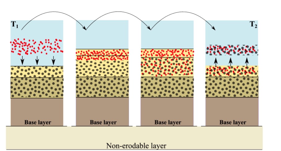
Fig. 6 Visualization of the diffusion that occurs when XBeach calculates sediment compositions. After sedimentation of fine sediment on top of coarser material it is uniformly mixed over the whole layer. Subsequent erosion erodes both the fines as the coarser material. To avoid this phenomenon, layers should not be too thick ([van der Zwaag, 2014]).
Ship-induced wave motions
See also
Ship-induced wave motions are implemented in mod:ship_module.
A relatively new application field for XBeach is the generation and propagation of waves induced by sailing vessels. This functionality has been implemented recently [Zhou et al., 2013], and has currently been used in several studies (e.g. [Zhou et al., 2014], [de Jong et al., 2013]), showing very good results.
For computing ship-induced waves the non-hydrostatic version of XBeach is used. A moving ship is represented as a pressure head that moves along a pre-defined track through the model domain. The ship is defined on a separate grid, where the ship draft is specified per grid point. Each computational time step the ship draft is interpolated from the ship grid to the global grid, where the ship volume is kept constant. Then the water pressure head in each global grid cell is updated based on the interpolated ship draft. By moving the pressure fields, the waves are generated and will propagate further through the global domain.
In fig-ship-example an example XBeach setup for ship waves is shown. The ship
track is user defined and can, for instance, be obtained from the
Automatic Identification System (AIS) for marine traffic. In this
example, the model results were compared with measurements taken at
Bath, The Netherlands. A filtered time series of the measured and
computed water level is shown in Fig. 7. The time series was
filtered to focus on the computation of the primary ship wave.
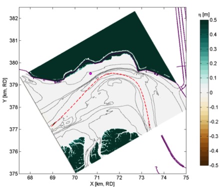
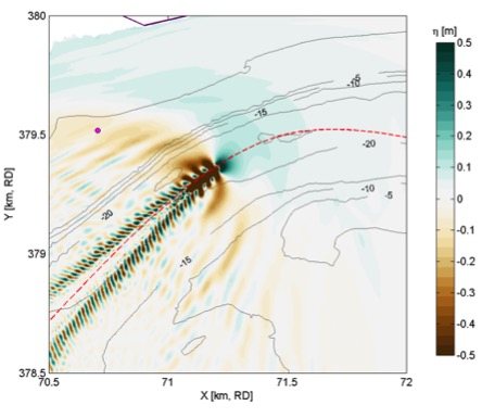
Example XBeach setup (left) and result (right) for a ship wave simulation in the Scheldt Estuary (The Netherlands). The ship track (red dashed line) is user-defined, and the measurement location is indicated (magenta dot).

Fig. 7 Example XBeach result for ship-induced waves. Measurements are taken at Bath, in the Scheldt Estuary, The Netherlands ([Schroevers et al., 2011]).
In addition to the propagation of ship-induced waves, XBeach computes the forces and moments acting on the ship body. With this functionality, passing ship effects can be analyzed (e.g. [Zhou et al., 2013]).
Gravel (XBeach-G)
XBeach-G was a branch of the main XBeach development that has been developed to simulate storm impacts on gravel beaches. The development of XBeach-G have been taking place as a joint collaboration between Plymouth University and Deltares, as part of the EPSRC-funded NUPSIG-project. The relevant XBeach-G formulations have been merged back into to the XBeach trunk for the XBeachX release (fall 2017). XBeach-G formulations can be activated with the keyword useXBeachGSettings = 1).
XBeach-G uses the one-layer, depth-averaged, non-hydrostatic extension to the XBeach model (nonh=1), which is similar to the SWASH model ([Zijlema et al., 2011]) to solve wave-by-wave flow and surface elevation variations due to short waves in intermediate and shallow water depths. This is particularly important for application on gravel beaches, where due to steep slopes swash motion is mainly at incident wave frequencies, and infragravity wave motion, which dominates the inner surf and swash zone on sandy beaches during storms, is of secondary importance. To correctly account for upper swash infiltration losses and exfiltration effects on lower swash hydrodynamics on gravel beaches, XBeach-G computes groundwater dynamics and the exchange between groundwater and surface water using the XBeach groundwater model (gwflow = 1). Again, interaction between swash flows and the beach groundwater table are considered particularly important on gravel beaches due to the relatively large hydraulic conductivity of the sediment, while on sandy beaches this process is of significantly less importance. Finally, gravel sediment transport processes (McCall & Van Rijn) have been included in XBeach-G to simulate the morphodynamics of gravel beaches during storms. These transport processes are currently under further development and validation.
For more information on XBeach-G, download the PhD thesis of McCall (2015) on URL: http://hdl.handle.net/10026.1/3929.
Boundary conditions
Waves
See also
Wave boundary conditions are implemented in mod:waveparams. The latest functionalities, like spatially varying spectral conditions are implemented in mod:spectral_wave_bc_module.
XBeach allows users to include two different options for wave boundary conditions in the model. These wave boundary conditions can be applied only at the seaward boundary (keyword: wbctype). First of all, in Spectral conditions the method to specify wave spectra is discussed. Secondly, in Non-spectral conditions the method to apply non-spectra, such as stationary wave conditions or time-series is elaborated. In Lateral boundary conditions the lateral boundary conditions for waves are discussed. There is currently not a possibility to force waves on the landward boundary of a model.
Spectral conditions
The most-used wave boundary condition in XBeach is a spectral type. The input description of spectral wave boundary conditions can be found in Spectral wave boundary conditions. XBeach allows the user to define these with three possibilities:
: With this option you define the boundary condition as parametric spectral input. The parameters (i.e. the spectral shape, the wave period and the directional spreading) can be specified. The option is especially handy when there is no nested model or measured spectrum. Here are two options:
: In this case the two-dimensional (frequency-direction) output by the spectral wave model SWAN (.sp2 files) can be specified. (keyword wbctype = swan). This option is especially convenient when nesting XBeach into a SWAN model.
: In this case a more general type spectrum can be specified. (keyword wbctype = vardens). This option is often used when a measured spectrum is available.
Non-spectral conditions
XBeach also allows the user to define non-spectral wave boundary conditions. This is a variation of both wave conditions without wave groups and time series. The input description of non-spectral wave boundary conditions can be found in Non-spectral wave boundary conditions. XBeach allows the user to define these with two possibilities:
This means that a uniform and constant wave energy is specified, based on the given values of \({H}_{rms}\), \({T}_{m01}\), direction and power of the directional distribution function. The station boundary condition will contain wave groups. Here there are two options:
. The user can also specify the variation in time of the wave energy. There are three options:
First-order time series of waves (keyword wbctype = ts_1). XBeach will calculate the bound long wave based on the theory of [Longuet-Higgins and Stewart, 1964]).
Second-order time series of waves (keyword wbctype = ts_2). The bound long wave is specified by the user via a long wave elevation.
It is also possible to specify a variation in time of the horizontal velocity, vertical velocity and the free surface elevation (keyword: wbctype = ts_nonh). Last two terms are optional in this boundary conditions type.
Special conditions
Besides clear spectral or non-spectral wave boundary conditions, there are also three special boundary condition types implemented in XBeach.
(keyword wbctype = bichrom). In this case, XBeach will be forced with regular wave groups as the two short-wave components force one difference (infragravity) wave period. The user needs to specify not only variables of the stationary situation but also a wave period for the long wave. This wave period will be used to calculate the long wave based on the theory of [Longuet-Higgins and Stewart, 1964]. The bichromatic boundary condition is the most simplified form of a wave spectrum.
(keyword wbctype = off). This is a simple no wave action boundary condition. It still allows for a tidal record to be specified, however this trough the zs0file parameter.
(keyword: wbctype = reuse). If the user does not wish to recalculate boundary condition files or specifically wants to reuse the boundary condition files of another XBeach simulation should be used. No further wave boundary condition data need be given. Obviously, the calculation grid should remain the same between runs, as the angles and number of grid points are embedded in the boundary condition files.
Lateral boundary conditions
There are two options to set the lateral boundaries for the wave model:
Neumann boundaries (keyword: lateralwave = neumann): here the longshore gradient is set to zero.
Wave crest boundaries (keyword: lateralwave = wavecrest). here the gradient in the wave energy along the wave crest is set to zero.
For the stationary wave mode (keyword: wavemodel = stationary) this is the only option. It allows a correct representation of the wave propagation near the lateral boundaries, without the usual shadow zones in e.g. SWAN. By neglecting the longshore gradients, the model automatically computes a consistent 1D solution.
For the surfbeat mode (keyword: wavemodel = surfbeat), Neumann leads to shadow zones, not so much in the wave height, but in the groupiness; the ‘blobs’ propagating in the mean wave direction turn into elongated, longshore uniform patches. To reduce this effect, the gradient along the wave crests of the wave energy can be set to zero, instead of the longshore gradient (keyword: lateralwave = wavecrest). This way the crests of the wave groups have approximately the right orientation, though the along-crest groupiness also disappears. In the wavecrest case, the wave refraction may be overestimated leading to somewhat too large longshore currents. The effects of both boundary conditions are shown in Fig. 8.
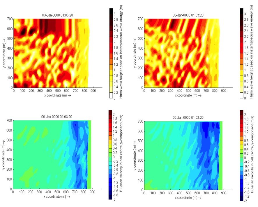
Fig. 8 Effect of the lateral wave boundary conditions on root-mean square wave height patterns (top) and longshore velocity (bottom) for the Delilah test case. In this figure the left panels are used for simulations with Neumann boundaries and the right panel with the wavecrest boundary.
Shallow water equations
Offshore boundary
Typically, an offshore or lateral boundary is an artificial boundary which has no physical meaning. On the offshore boundary wave and flow conditions are imposed. In the domain waves and currents will be generated which need to pass through the offshore boundary to the deep sea with minimal reflection. One way to do this is to impose a weakly reflective-type boundary condition (absorbing-generating), but there are also other possibilities implemented in XBeach (keyword: front). This method can be applied in 1D or 2D, is recommended and therefore the default value for XBeach.
In XBeach, there are two options with regard to the offshore absorbing-generating boundary condition. With the parameter setting front = abs1d a simple one-dimensional absorbing-generating boundary condition is activated. This option allows for a time-varying water level (surge and/or infragravity waves) to be specified at the boundary while allowing any waves propagating perpendicularly towards the boundary to be absorbed (i.e., passed through the boundary with a minimum of reflection. It is therefore only useful for 1D (flume like) simulations.
With option front = abs2d (default value) the formulation by [van Dongeren and Svendsen, 1997] is activated which in turn is based on [Verboom et al., 1981] and is based on the ‘Method of Characteristics’. This boundary condition allows for obliquely-incident and obliquely-reflected waves to pass through the boundary. It is possible to account for situations with boundary-perpendicular and boundary-parallel currents. In order to differentiate between the particle velocities, the keyword epsi must be set. This parameter control a simple Kalman-update filter which controls which part of the particle velocity is assumed to be part of the current and which part is wave-related. By default XBeach computes the value for epsi automatically using offshore boundary conditions (keyword: epsi = -1).
There are three other possibilities implemented besides the absorbing-generating boundary conditions:
No flux wall (keyword: front = wall). This boundary condition type is a simple no flux boundary condition.
Water level specification (keyword: front = wlevel). This boundary sets the water level at a prescribed value. This can be constant or time-varying. With this option the outgoing long waves are not absorbed.
Boundary condition for the non-hydrostatic option (keyword: : front = nonh_1d). This boundary condition is required for non-hydrostatic simulations.
Radiation boundary condition (keyword: front = waveflume). This boundary uses a continuity relation at the front boundary. This means that no net water can come into the model domain. The wave flume boundary condition is especially useful in lab experiments with a large set-up (e.g. coral reefs).
Lateral boundaries
Lateral boundaries are the boundaries perpendicular to the coastline. Usually these are artificial, because the model domain is limited but the physical coast will continue. At these boundaries (keywords: left & right) we need to prescribe information about the area beyond the numerical model domain in such a way that the boundary condition does not influence the results in an adverse way. One way to do this is to prescribe a so-called ‘no-gradient’ or Neumann boundaries (XBeach default), which state that there is locally no change in surface elevation and velocity, but there are also other possibilities implemented into XBeach. This method is recommended and is therefore the default value for XBeach. Each lateral boundary is a separate condition, so it is possible to mix different type of lateral boundary per side.
Neumann boundary conditions are activated where the longshore water level gradient is prescribed. The alongshore gradient is prescribed by the difference in specified water levels at the offshore corner points, divided by the alongshore length of the domain. This type of Neumann boundary condition has been shown to work quite well with (quasi-) stationary situations, where the coast can be assumed to be uniform alongshore outside the model domain. So far we have found that also in case of obliquely incident wave groups this kind of boundary conditions appears to give reasonable results when a shadow zone is taken into account. This means that regions where the boundary conditions are not fully enforced the results are not taken into account. Neumann boundaries can be individually defined (keyword: left = neumann).
There are three other possibilities implemented besides the absorbing-generating boundary conditions:
Simple no-flux boundary conditions can also be applied (keyword: left = wall). Wall boundary conditions will result in a zero velocity at the lateral boundary.
Velocity at the boundary will be calculated from NLSWE, but only include the advective terms (keywords: left = no_advec). The effect is that only terms that decrease the velocity will be taken into account. The result is an intermediate form between a full Neumann boundary and a wall boundary.
Velocity at the boundary will simply be copied from the adjacent cell in the model domain (keyword: left = neumann_v).
Tide and surge
XBeach can take in up to four time-vary tidal signals to be applied to the four boundaries (offshore-right, offshore-left, backshore-left, backshore-right). A time-varying water level signal is read into XBeach by reading the specified file in zs0file. The input signal will be interpolated to the local time step of the simulation; therefore the signals only need to be long enough and temporally-fine enough to resolve the water level phenomenon of interest (i.e. tide variations, surge event).
There are now four options for handling the tidal and/or surge contribution to the boundaries:
Uniform water level (keyword: tideloc = 0)
One time-varying water level signal (keyword: tideloc = 1)
Two time-varying water level signals, which requires point of application indication. (keyword: tideloc = 2)
Four time-varying water level signals (keyword: tideloc = 4)
For the option with a uniform water level the value specified in the params.txt is applied in the complete model domain (keyword: zs0). For the option with one time-varying water level signal the specified water level is applied (keyword: zs0file = <name_of_your_time_series_file>) to the offshore boundary and a fixed value is applied at the backshore boundary (keyword: zs0). For the option with two time-varying water level signals two water level signals are read from the zs0file. Note: one tidal record is applied to both sea corners and one tidal record to both land corners. This means there is no alongshore variation. An alongshore variation can be applied when applying four time-varying water level signals.
River and point discharge
The effect of a river outflow or other discharges can be simulated with XBeach. Multiple discharge locations can be designated. At a discharge location the discharge orifice is defined as well as the discharge time series in \({\rm m}^{3}/{\rm s}\). The discharge orifice always constitutes an uninterrupted series of full grid abreast cell borders. It is not possible to define a discharge over half a grid cell nor is it possible to define a single discharge through grid cell borders that are either not adjacent or are not abreast.
At each time step the model sets the discharge and velocities at the grid cell borders that constitute the discharge orifice, which can be computed given the size of the discharge orifice and discharge time series. The discharge is positive in positive x or y direction. An exception is made when discharges are defined at the domain border. In that case the discharge is positive towards the domain (influx).
When a discharge is defined with a zero size orifice the discharge is assumed to be in vertical direction where a positive discharge is into the domain (influx). In these cases the discharge is linked to the closest grid cell center and at each time step mass according to the discharge time series is added. No momentum is added in case of a vertical discharge.
Sediment transport
The boundary conditions for sediment transport are Neumann boundaries everywhere, implying that the cross-boundary gradients in the advection-diffusion equation are set to zero, as well as the gradients of the bed load transports in that direction. Cross-shore profile changes due to cross-shore transport gradients are possible, allowing the boundary to smoothly follow the rest of the model. Still, it is good modeling practice to have the boundaries away from the area of interest.
Input description
General
Upon running the XBeach executable xbeach.exe, the file params.txt in the current working directory will be read. The params.txt file contains grid and bathymetry info, wave input, flow input, morphological input, etc. in the form of keyword/value pairs. Each keyword/value pair may contain an actual model parameter or refer to another file with additional information on the model setup. If a params.txt file cannot be found then XBeach will not run.
In the params.txt file there can be a single keyword/value pair per line. The keywords can be specified in any order. A keyword/value pair is separated by an equal sign (=). Each line containing an equal sign is interpreted as a keyword/value pair. Reversely, any lines without an equal sign are ignored and may be used for comments. Only a few keywords are required for the model to run, others have default values that are used in case the keyword is not mentioned in the params.txt file. The essential parameters for a simulation with a JONSWAP spectrum are listed below:
A . This can both in XBeach format (separate x and y files; keyword: xfile and yfile) or Delft3D (one single xy file; keyword: xyfile). On top of that the user needs to specify the width of each domain (keyword: nx and ny)
A file (keyword: depfile) that matches with the grid you specified at 1)
A (keyword: tstop) in seconds
A for short waves and rollers. The grid is determined by a minimum and maximum angle and width per bin (keywords: thetamin, thetamax and dtheta).
A (keyword: wbctype = jons). With a separate file containing the variables of the parametric (keyword: bcfile).
It is strongly recommended to specify as few parameters explicitly as possible and rely on the defaults for the other parameters. When running XBeach, a file called xbeach.log is created, which lists all the parameters set through the params.txt file but also all parameters not set, for which the defaults are used. When the user starts the model, it generates a file named XBlog.txt. In this file all the different keyword available are determined. When no keyword is defined the default value will be applied.
This chapter describes the possibilities of the params.txt file and any auxiliary information files that are called from the params.txt file. The tables in this chapter contain a description of the keywords, the default values, its units and recommended value ranges, while the formats for additional input files are described in the relevant sections. Keyword marked with an astrix (*) are essential for XBeach to run. Keywords marked with a plus (+) are considered advanced expert options and should not be used for regular applications of XBeach.
In this chapter, any references to keywords refer to keywords that can be used in the params.txt file. Also any references to time indications are in seconds unless stated otherwise. A typical params.txt file for a 1D XBeach model is:
params.txt
%%%%%%%%%%%%%%%%%%%%%%%%%%%%%%%%%%%%%%%%%%%%%%%%%%%%%%%%%%%%%%%%%%%%%%%%%%%
%%% XBeach parameter settings input file                                %%%
%%%                                                                     %%%
%%% date: 01-Jan-2015 12:00                                             %%%
%%% function: xb_write_params                                           %%%
%%%%%%%%%%%%%%%%%%%%%%%%%%%%%%%%%%%%%%%%%%%%%%%%%%%%%%%%%%%%%%%%%%%%%%%%%%%

%%% Grid parameters %%%%%%%%%%%%%%%%%%%%%%%%%%%%%%%%%%%%%%%%%%%%%%%%%%%%%%%

depfile = bed.dep
posdwn = 0
nx = 265
ny = 0
alfa = 0
vardx = 1
xfile = x.grd
yfile = y.grd
thetamin = -90
thetamax = 90
dtheta = 15
thetanaut = 0

%%% Model time %%%%%%%%%%%%%%%%%%%%%%%%%%%%%%%%%%%%%%%%%%%%%%%%%%%%%%%%%%%%

tstop = 3600

%%% Physical constants %%%%%%%%%%%%%%%%%%%%%%%%%%%%%%%%%%%%%%%%%%%%%%%%%%%%

rho = 1025

%%% Tide boundary conditions %%%%%%%%%%%%%%%%%%%%%%%%%%%%%%%%%%%%%%%%%%%%%%

tideloc = 2
zs0file = tide.txt

%%% Wave boundary condition parameters %%%%%%%%%%%%%%%%%%%%%%%%%%%%%%%%%%%%

wbctype = jons
bcfile = filelist.txt

%%% Output variables %%%%%%%%%%%%%%%%%%%%%%%%%%%%%%%%%%%%%%%%%%%%%%%%%%%%%%

outputformat = netcdf
tint = 3600
tstart = 0
nglobalvar = 3
zb
zs
H
Physical processes
XBeach supports a variety of physical processes from generic, like waves and flow, to very specific, like ship motions and point discharge. Each process can be switched on or off. The commonly used processes are turned on by default. The table below lists the keywords used to switch on or off physical processes in XBeach.
parameter |
description |
default |
range |
units |
|---|---|---|---|---|
advection |
Include advection in flow solver |
1 |
0 - 1 |
|
avalanching |
Turn on avalanching |
1 |
0 - 1 |
|
cyclic |
Turn on cyclic boundary conditions |
0 |
0 - 1 |
|
flow |
Turn on flow calculation |
1 |
0 - 1 |
|
gwflow+ |
Turn on groundwater flow |
0 |
0 - 1 |
|
lwave |
Turn on short wave forcing on nlsw equations and boundary conditions |
1 |
0 - 1 |
|
morphology |
Turn on morphology |
0 |
0 - 1 |
|
nonh+ |
Turn on non-hydrostatic pressure: 0 = nswe, 1 = nsw + non-hydrostatic pressure compensation stelling & zijlema, 2003 |
0 |
0 - 1 |
|
q3d |
Turn on quasi-3d sediment transport |
0 |
0 - 1 |
|
sedtrans |
Turn on sediment transport |
1 |
0 - 1 |
|
setbathy |
Turn on timeseries of prescribed bathy input |
0 |
0 - 1 |
|
ships+ |
Turn on ship waves |
0 |
0 - 1 |
|
single_dir+ |
Turn on stationary model for refraction, surfbeat based on mean direction |
1 |
0 - 1 |
|
snells+ |
Turn on snell’s law for wave refraction |
0 |
0 - 1 |
|
swave |
Turn on short waves |
1 |
0 - 1 |
|
swrunup |
Turn on short wave runup |
0 |
0 - 1 |
|
vegetation+ |
Turn on interaction of waves and flow with vegetation |
0 |
0 - 1 |
|
viscosity |
Include viscosity in flow solver |
1 |
0 - 1 |
|
wavemodel |
Stationary (0), surfbeat (1) or non-hydrostatic (2) |
surfbeat |
stationary, surfbeat, nonh |
|
wind |
Include wind in flow solver |
1 |
0 - 1 |
Grid and bathymetry
XBeach spatial grid size is defined by the keywords nx and ny. Here nx are the number of grid points in the cross-shore direction and ny the number in the alongshore direction. The size of the computational grid will be nx +1 by ny +1 cells large. The initial bathymetry is provided using a separate file that is referred to by the depfile keyword, which has to have a size of [nx+1, ny+1]. This file contains an initial bed level for each grid cell where each line corresponds to a transect in x-direction (cross-shore). The values are positive down by default (so e.g. a value of ‘10’ is 10 meters depth), but this can be changed using the posdwn keyword.
Three main types of XBeach grids are supported: fast 1D, 1D and 2DH. Fast 1D grids have a single alongshore grid cell and thus a value ny = 0 and thus a single row (ny+1=1) in the depfile. The 1D grids have 3 alongshore grid cells and thus a value ny = 2 and three rows in the depfile. The 2DH grids have more than 3 alongshore grid cells, a value ny >2 and as many rows in the depfile. In general, the bathymetry file has the following space-separated format:
bed.dep
<z 1,1> <z 2,1> <z 3,1> ... <z nx,1> <z nx+1,1>
<z 1,2> <z 2,2> <z 3,2> ... <z nx,2> <z nx+1,2>
<z 1,3> <z 2,3> <z 3,3> ... <z nx,3> <z nx+1,3>

...

<z 1,ny> <z 2,ny> <z 3,ny> ... <z nx,ny> <z nx+1,ny>
<z 1,ny+1> <z 2,ny+1> <z 3,ny+1> ... <z nx,ny+1> <z nx+1,ny+1>
XBeach spatial grids can be equidistant or non-equidistant. In the former case the grid size is defined by the keywords dx and dy. In the latter case the keyword vardx should be set to 1 and x- and y-coordinates of the grid cells should be provided through the files referenced by the xfile and yfile keywords. These files take exactly the same format as the depfile file where all coordinates along the x-direction are in one row and each row represents a cell in y-direction. XBeach grids are defined in a coordinate system of choice and can be either rectangular or curvilinear grids as discussed in Domain and definitions.
Delft3D grids created with tools like RFGRID are also supported. To use Delft3D grids, choose gridform = delft3d and provide a grid file via the keyword xyfile. The format of Delft3D grids is not described here, but can be found in the Delft3D manual ([Deltares, 2011]). Also forced updating of bathymetries is supported as described in Bed update.
Apart for the spatial grid, XBeach also uses a directional grid for short waves and rollers. The grid is determined by a minimum and maximum angle and a directional bin size using the keywords thetamin, thetamax and dtheta respectively. The thetamin and thetamax angles are either defined according to the Cartesian convention (angle w.r.t. the computational x-axis) or according to the nautical convention (angle w.r.t. deg. N, so from W is 270 deg. N). The convention is chosen using the keyword thetanaut (thetanaut = 0 for Cartesian and thetanaut = 1 for Nautical)
Examples of typical input for a non-equidistant, fast 1D XBeach model, together with the params.txt example at the start of this chapter, are:
depfile = bed.dep
-20.00 -20.00 -19.90 -19.80 -19.70 ... 14 14 15 15 15
xfile = x.grd
0.00 10.00 20.00 30.00 40.00 ... 1992.00 1994.00 1996.00 1998.00 2000.00
yfile = y.grd
0.00 0.00 0.00 0.00 0.00 0.00 0.00 ... 0.00 0.00 0.00 0.00 0.00 0.00 0.00
All keywords related to grid and bathymetry input are listed in the following table:
parameter |
description |
default |
range |
units |
|---|---|---|---|---|
alfa |
Angle of x-axis from east |
0.0 |
0.0 - 360.0 |
deg |
depfile* |
Name of the input bathymetry file |
<file> |
||
dtheta* |
Directional resolution |
10.0 |
0.1 - 180.0 |
deg |
dtheta_s* |
Directional resolution in case of stationary refraction |
10.0 |
0.1 - 20.0 |
deg |
dx* |
Regular grid spacing in x-direction |
-1.0 |
0.0 - 1000000000.0 |
m |
dy* |
Regular grid spacing in y-direction |
-1.0 |
0.0 - 1000000000.0 |
m |
gridform |
Grid definition format |
xbeach |
xbeach, delft3d |
|
nx* |
Number of computational cell corners in x-direction |
50 |
2 - 10000 |
|
ny* |
Number of computational cell corners in y-direction |
2 |
0 - 10000 |
|
nz |
Number of computational cells in z-direction |
1 |
1 - 100 |
|
posdwn |
Bathymetry is specified positive down (1) or positive up (-1) |
1.0 |
-1.0 - 1.0 |
|
thetamax* |
Higher directional limit (angle w.r.t computational x-axis) |
90.0 |
-360.0 - 360.0 |
deg |
thetamin* |
Lower directional limit (angle w.r.t computational x-axis) |
-90.0 |
-360.0 - 360.0 |
deg |
thetanaut |
Switch to specify thetamin and thetamax in nautical convention rather than cartesian |
0 |
0 - 1 |
|
vardx |
Switch for variable grid spacing |
0 |
0 - 1 |
|
xfile |
Name of the file containing x-coordinates of the calculation grid |
<file> |
||
xori |
X-coordinate of origin of axis |
0.0 |
-1000000000.0 - 1000000000.0 |
m |
xyfile* |
Name of the file containing delft3d xy-coordinates of the calculation grid |
<file> |
||
yfile |
Name of the file containing y-coordinates of the calculation grid |
<file> |
||
yori |
Y-coordinate of origin of axis |
0.0 |
-1000000000.0 - 1000000000.0 |
m |
Waves input
An XBeach model is generally forced by waves on its offshore boundary. These waves are described by the wave boundary conditions discussed in this section. The details of the wave motions within the model are described by the wave numerics in terms of the wave action balance (see Short wave action balance), wave dissipation model (see 0) and wave roller model (see Roller energy balance)
XBeach supports a variety of wave boundary condition types that are divided in two main groups: stationary and spectral boundary conditions. The wbctype keyword can be used to select one particular type of wave boundary conditions. Waves gives an overview of all types of wave boundary conditions available for XBeach. Fig. 9 can be used to help determine what type of wave boundary conditions is appropriate for your case. Each wave boundary condition type is explained in the following subsections. Note that most spectral wave boundary conditions can vary both in space and time using a FILELIST and/or LOCLIST construction as described in Temporally and/or spatially varying wave boundary conditions.
parameter |
description |
default |
range |
units |
|---|---|---|---|---|
Hrms |
Hrms wave height for instat = stat, bichrom, ts_1 or ts_2 |
1.0 |
0.0 - 10.0 |
m |
Tlong |
Wave group period for case instat = bichrom |
80.0 |
20.0 - 300.0 |
s |
Trep |
Representative wave period for instat = stat, bichrom, ts_1 or ts_2 |
10.0 |
1.0 - 20.0 |
s |
dir0 |
Mean wave direction for instat = stat, bichrom, ts_1 or ts_2 (nautical convention) |
270.0 |
-360.0 - 360.0 |
deg |
instat |
Old wave boundary condition type |
bichrom |
stat, bichrom, ts_1, ts_2, jons, swan, vardens, reuse, ts_nonh, off, stat_table, jons_table |
|
lateralwave |
Switch for lateral boundary at left |
neumann |
neumann, wavecrest, cyclic |
|
m |
Power in cos^m directional distribution for instat = stat, bichrom, ts_1 or ts_2 |
10 |
2 - 128 |
|
taper |
Spin-up time of wave boundary conditions, in morphological time |
100.0 |
0.0 - 1000.0 |
s |
wbctype |
New wave boundary condition type |
jonstable |
params, parametric, swan, vardens, off, jonstable, reuse, ts_1, ts_2, ts_nonh |
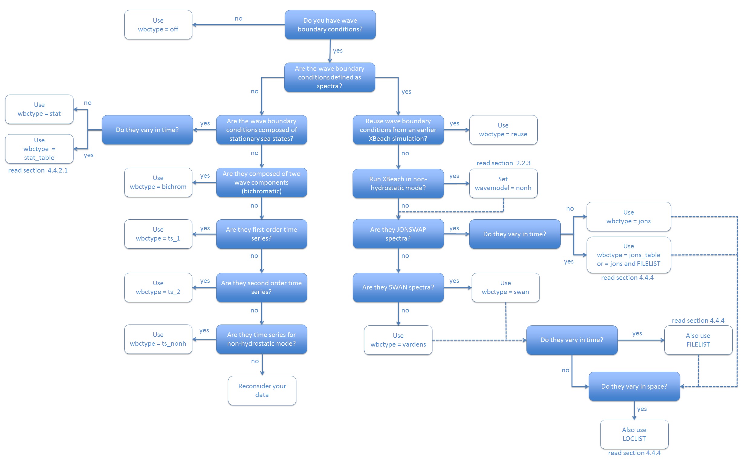
Fig. 9 Decision tree for selecting the appropriate type of wave boundary conditions
Spectral wave boundary conditions
Spectral wave boundary conditions are enabled using wbctype values jons, swan, vardens or jons_table. The conditions are defined in separate files referenced from the params.txt file using the bcfile keyword. A spectral wave boundary condition describes a spectrum shape that XBeach uses to generate a (random) wave time series. The length and resolution of the generated time series is determined by the keywords rt and dtbc respectively. XBeach will reuse the generated time series until the simulation is completed. The resolution of the time series should be enough to accurately represent the bound long wave, but need not be as small as the time step used in XBeach.
An overview of all keywords relevant for spectral wave boundary conditions is given in the table below. The necessary file formats for each type of spectral wave boundary condition is explained in the following subsections.
parameter |
description |
default |
range |
units |
|---|---|---|---|---|
Tm01switch+ |
Switch to enable tm01 rather than tm-10 |
0 |
0 - 1 |
|
bcfile |
Name of spectrum file |
<file> |
||
correctHm0 |
Switch to enable hm0 correction |
1 |
0 - 1 |
|
dtbc+ |
Timestep used to describe time series of wave energy and long wave flux at offshore boundary (not affected by morfac) |
1.0 |
0.1 - 2.0 |
s |
dthetaS_XB+ |
The (counter-clockwise) angle in the degrees needed to rotate from the x-axis in swan to the x-axis pointing east |
0.0 |
-360.0 - 360.0 |
deg |
fcutoff+ |
Low-freq cutoff frequency for instat = jons, swan or vardens boundary conditions |
0.0 |
0.0 - 40.0 |
Hz |
nonhspectrum+ |
Spectrum format for wave action balance of nonhydrostatic waves |
0 |
0 - 1 |
|
nspectrumloc+ |
Number of input spectrum locations |
1 |
1 - par%ny+1 |
|
nspr |
Switch to enable long wave direction forced into centres of short wave bins |
0 |
0 - 1 |
|
random+ |
Switch to enable random seed for instat = jons, swan or vardens boundary conditions |
1 |
0 - 1 |
|
rt |
Duration of wave spectrum at offshore boundary, in morphological time |
min(3600.d0,par%tstop) |
1200.0 - 7200.0 |
s |
sprdthr+ |
Threshold ratio to maximum value of s above which spectrum densities are read in |
0.08 |
0.0 - 1.0 |
|
trepfac+ |
Compute mean wave period over energy band: par%trepfac*maxval(sf) for instat jons, swan or vardens; converges to tm01 for trepfac = 0.0 and |
0.01 |
0.0 - 1.0 |
|
wbcversion |
Version of wave boundary conditions |
3 |
1 - 3 |
JONSWAP wave spectra
JONSWAP spectrum input is enabled using wbctype = jons. A JONSWAP wave spectrum is parametrically defined in a file that is referenced using the bcfile keyword. This file contains a single parameter per line in arbitrary order. The parameters that can be defined are listed in Table 8. All variables are optional. If no value is given, the default value as specified in the table is used. It is advised not to specify the keyword dfj and allow XBeach to calculate the default value.
A typical JONSWAP definition file looks as follows:
jonswap.txt
Hm0 = 0.8
Tp = 8
mainang = 285.
gammajsp = 3.3
s = 10.
fnyq = 0.3
For the definitions see the table below.
It is possible to use an alternative file format for time-varying JONSWAP spectra. To enable this option use the wbctype value jons_table. In this case, each line in the spectrum definition file contains a parametric definition of a spectrum, like in a regular JONSWAP definition file, plus the duration for which that spectrum is used during the simulation. XBeach does not reuse time-varying spectrum files. Therefore the total duration of all spectra should at least match the duration of the simulation. The name of the file can be chosen freely, but the file format is fixed as follows and all parameters should be present in all lines:
jonswap.txt
<Hm0> <Tp> <mainang> <gammajsp> <s> <duration> <dtbc>
Note that we refer to the keywords used in a regular JONSWAP definition file in this example, with three differences: 1) the peak period rather than the peak frequency is defined 2) the duration is added (similar to rt in params.txt) 3) the time resolution is added (similar to dtbc in params.txt). The duration and boundary condition time step in this file overrules rt and dtbc in params.txt. This format is also used for time-varying stationary wave boundary conditions as described in Temporally and/or spatially varying wave boundary conditions. As an example, the JONSWAP spectrum definition file presented above would look as follows if the significant wave height should be increased with 0.2 m every hour:
jonswap.txt
0.8 8. 285. 3.3 10. 3600. 1
1.0 8. 285. 3.3 10. 3600. 1
1.2 8. 285. 3.3 10. 3600. 1
A more generic way of providing time-varying spectral wave boundary conditions is using a FILELIST construction as described in Temporally and/or spatially varying wave boundary conditions. This approach is compatible with all spectral wave boundary condition types as well as spatially varying boundary conditions as described in the same section.
The parameter s in the JONSWAP spectrum definition is related to the directional spreading in radians through the following relation:
\(\sigma (radians) = \sqrt{\frac{2}{s+1} }\)
and in degrees:
\(\sigma (degrees) = \frac{180}{\pi} \sqrt{\frac{2}{s+1} }\)
Similarly, s can be calculated from \(\sigma\) as:
\(s=\frac{2}{\sigma ^{2} } -1\).
Here \(\sigma\) is the directional spreading in radians and s the JONSWAP spreading parameter.
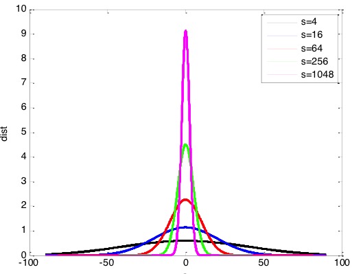
Fig. 10 Effect a variation in s for the direction spreading of wave energy
parameter |
description |
default |
range |
units |
|---|---|---|---|---|
Hm0 |
Hm0 of the wave spectrum, significant wave height [m] |
0.0 |
0.0 - 5.0 |
|
fp |
Peak frequency of the wave spectrum [s-1] |
0.08 |
0.06258 - 0.4 |
|
gammajsp |
Peak enhancement factor in the JONSWAP expression [-] |
3.3 |
1.0 - 5.0 |
|
s |
Directional spreading coefficient, {cos}^{2s} law [-] |
10.0 |
1.0 - 1000.0 |
|
mainang |
Main wave angle (nautical convention) [{}^circ] |
270.0 |
180.0 - 360.0 |
|
fnyq |
Highest frequency used to create JONSWAP spectrum [s-1] |
0.3 |
0.2 - 1.0 |
|
dfj |
Step size frequency used to create JONSWAP spectrum [s-1] |
fnyq/200 |
fnyq/1000 - fnyq/20 |
SWAN wave spectra
XBeach can read standard SWAN 2D variance density or energy density output files (+.sp2 files) as specified in the SWAN v40.51 manual. This option is enabled using wbctype = swan in params.txt and a reference to the spectrum file via the keyword bcfile. XBeach assumes the directional information in the SWAN file is according to the nautical convention. If the file uses the Cartesian convention for directions, the user must specify the angle in degrees to rotate the x-axis in SWAN to the x-axis in XBeach (by the Cartesian convention). This value is specified in params.txt using the keyword dthetaS_XB.
Note that time-varying and spatially varying SWAN spectra can be provided using the FILELIST and LOCLIST constructions as described in Temporally and/or spatially varying wave boundary conditions.
An example of a 2D SWAN spectrum is given below:
swan.txt
SWAN 1 Swan standard spectral file
$ Data produced by SWAN version 40.51
$ Project:’projname’ ; run number:’runnum’
LOCATIONS locations in x-y-space
1 number of locations
22222.22 0.00
RFREQ relative frequencies in Hz
23 number of frequencies
0.0545
0.0622
0.0710
0.0810
0.0924
0.1055
0.1204
0.1375
0.1569
0.1791
0.2045
0.2334
0.2664
0.3040
0.3470
0.3961
0.4522
0.5161
0.5891
0.6724
0.7675
0.8761
1.0000
CDIR spectral Cartesian directions in degr 12 number of directions
30.0000
60.0000
90.0000
120.0000
150.0000
180.0000
210.0000
240.0000
270.0000
300.0000
330.0000
360.0000
QUANT 1 number of quantities in table VaDens variance densities in m2/Hz/degr m2/Hz/degr unit
-0.9900E+02 exception value
FACTOR
0.675611E-06
51 242 574 956 1288 1482 1481 1286 957 579 244 51
129 610 1443 2402 3238 3725 3724 3234 2406 1454 613 128
273 1287 3054 5084 6846 7872 7869 6837 5091 3076 1295 271
665 3152 7463 12402 16712 19229 19221 16690 12419 7518 3172 662
1302 6159 14608 24275 32688 37618 37603 32644 24309 14716 6198 1296
2328 10989 26020 43341 58358 67109 67080 58281 43401 26213 11058 2317
3365 15922 37712 62733 84492 97150 97110 84380 62820 37991 16021 3349
3426 16230 38440 63939 86109 99010 98969 85995 64027 38724 16331 3410
2027 9612 22730 37790 50909 58529 58505 50841 37843 22898 9672 2018
672 3178 7538 12535 16892 19440 19432 16870 12552 7594 3198 669
101 479 1135 1890 2542 2924 2923 2539 1892 1144 482 101
2 11 26 43 57 66 66 57 43 26 11 2
0 0 0 0 0 0 0 0 0 0 0 0
0 0 0 0 0 0 0 0 0 0 0 0
0 0 0 0 0 0 0 0 0 0 0 0
0 0 0 0 0 0 0 0 0 0 0 0
0 0 0 0 0 0 0 0 0 0 0 0
0 0 0 0 0 0 0 0 0 0 0 0
0 0 0 0 0 0 0 0 0 0 0 0
0 0 0 0 0 0 0 0 0 0 0 0
0 0 0 0 0 0 0 0 0 0 0 0
0 0 0 0 0 0 0 0 0 0 0 0
0 0 0 0 0 0 0 0 0 0 0 0
0 0 0 0 0 0 0 0 0 0 0 0
Variance density spectra
2D spectral information that is not in SWAN format can be provided using a formatted variance density spectrum file and wbctype = vardens. The spectrum file itself is again referenced using the keyword bcfile. The contents of the file must adhere to a specific format:
vardens.txt
<number of frequencies (n)>
<frequency 1>
<frequency 2>
<frequency 3>

...

<frequency n-1>
<frequency n>
<number of directions (m)>
<directions 1>
<directions 2>
<directions 3>

...

<directions m-1>
<directions m>
<variance density 1,1> <variance density 2,1> ... <variance density m,1>
<variance density 1,2> <variance density 2,2> ... <variance density m,2>

...

<variance density 1,n> <variance density 2,n> ... <variance density m,n>
Note that the directions must be defined according to the Cartesian convention and in the coordinate system used by XBeach. In this coordinate system \({0}^\circ\) corresponds to waves travelling in the direction of the x-axis, while \({90}^\circ\) corresponds to the direction of the y-axis. Also, the directions must be defined in increasing order. Time-varying and spatially varying variance density spectra can be provided using the FILELIST and LOCLIST constructions as described in Temporally and/or spatially varying wave boundary conditions.
An example of a formatted variance density file is given below:
vardens.txt
15
0.0418
0.0477
0.0545
0.0622
0.0710
0.0810
0.0924
0.1055
0.1204
0.1375
0.1569
0.1791
0.2045
0.2334
0.2664
13
-180.0000
-150.0000
-120.0000
-90.0000
-60.0000
-30.0000
0.0000
30.0000
60.0000
90.0000
120.0000
150.0000
180.0000
0 0 0 0 0 0 0 0 0 0 0 0
51 242 574 956 1288 1482 1481 1286 957 579 244 51
129 610 1443 2402 3238 3725 3724 3234 2406 1454 613 128
273 1287 3054 5084 6846 7872 7869 6837 5091 3076 1295 271
665 3152 7463 12402 16712 19229 19221 16690 12419 7518 3172 662
1302 6159 14608 24275 32688 37618 37603 32644 24309 14716 6198 1296
2328 10989 26020 43341 58358 67109 67080 58281 43401 26213 11058 2317
3365 15922 37712 62733 84492 97150 97110 84380 62820 37991 16021 3349
3426 16230 38440 63939 86109 99010 98969 85995 64027 38724 16331 3410
2027 9612 22730 37790 50909 58529 58505 50841 37843 22898 9672 2018
672 3178 7538 12535 16892 19440 19432 16870 12552 7594 3198 669
101 479 1135 1890 2542 2924 2923 2539 1892 1144 482 101
2 11 26 43 57 66 66 57 43 26 11 2
0 0 0 1 1 1 1 1 1 0 0 0
0 0 0 0 0 0 0 0 0 0 0 0
0 0 0 0 0 0 0 0 0 0 0 0
Reduction of short-wave group variance to include the effects of directional spreading in a 1-dimensional model
Infragravity wave growth is affected by the directional spreading of the short-waves. A wave field with directional spreading result in a lower infragravity wave height than a wave field with no directional spreading. Since directional spreading can only be modelled in a 2-dimensional model, the infragravity wave is overestimated in a 1-dimensional model. Even when boundary conditions including directional spreading are applied in a 1-dimensional model, the internal forcing inside the domain result in a larger infragravity wave compared to a 2-dimensional model with directional spreading. Infragravity wave growth in the XBeach model is controlled by wave forcing terms in the non-linear shallow water equations solved in the XBeach flow module. As such, there is no simple source or sink infragravity energy balance term available to tune in a modified 1D approach. Instead, infragravity wave heights can either be modified by dissipating infragravity waves more strongly (i.e., through increased viscosity or bed roughness), or by reducing the mechanisms for infragravity wave growth. Of these two options, increased dissipation through higher viscosity or bed roughness has the drawback of slowing flow in general, leading to increased predictions of wave set-up at the coast. Therefore, a correction factor on the mechanisms of infragravity wave growth is implemented.
To include the effects of directional spreading in a 1-dimensional model, a reduction parameter in the short-wave group variance is implemented (keyword wbcevarreduce). In this way, time- and space-varying radiation stress gradients are reduced, leading to less energy transfer to the infragravity waves, and hence smaller, more realistic infragravity waves. If the mean wave height remains unchanged, the model will still accurately predict mean circulations and setup.
The boundary signal of the wave groups is now given by:
where \(E_{old}\) is the computed short-wave energy time series at the boundary and \(\langle ... \rangle\) represent the averaging operator over the entire time series.
Non-spectral wave boundary conditions
Stationary wave boundary conditions are enabled using wbctype values stat, ts_1, ts_2, ts_nonh or stat_table. The conditions are generally defined within the params.txt file directly using the keywords described in the table below. In addition, in case of wbctype values ts_1 or ts_2 the file bc/gen.ezs should be present that describes the infragravity wave forcing generated outside of XBeach. For the wbctype ts_nonh also a separate file is needed. More information about these files in Non-spectral wave boundary conditions.
Stationary wave boundary conditions
Only in case of wbctype = stat_table the time-varying stationary wave boundary conditions are fully described in an external file referenced by the bcfile keyword. The bcfile keyword is part of the spectral wave boundary condition input and also the referenced file is designed for time-varying spectral input in the form of JONSWAP spectra (see Spectral wave boundary conditions). In stationary mode only the relevant data from this file is used and irrelevant data like gamma and dfj are discarded.
parameter |
description |
default |
range |
units |
|---|---|---|---|---|
Hrms |
Hrms wave height for instat = stat, bichrom, ts_1 or ts_2 |
1.0 |
0.0 - 10.0 |
m |
Tlong |
Wave group period for case instat = bichrom |
80.0 |
20.0 - 300.0 |
s |
Trep |
Representative wave period for instat = stat, bichrom, ts_1 or ts_2 |
10.0 |
1.0 - 20.0 |
s |
dir0 |
Mean wave direction for instat = stat, bichrom, ts_1 or ts_2 (nautical convention) |
270.0 |
-360.0 - 360.0 |
deg |
instat |
Old wave boundary condition type |
bichrom |
stat, bichrom, ts_1, ts_2, jons, swan, vardens, reuse, ts_nonh, off, stat_table, jons_table |
|
lateralwave |
Switch for lateral boundary at left |
neumann |
neumann, wavecrest, cyclic |
|
m |
Power in cos^m directional distribution for instat = stat, bichrom, ts_1 or ts_2 |
10 |
2 - 128 |
|
taper |
Spin-up time of wave boundary conditions, in morphological time |
100.0 |
0.0 - 1000.0 |
s |
wbctype |
New wave boundary condition type |
jonstable |
params, parametric, swan, vardens, off, jonstable, reuse, ts_1, ts_2, ts_nonh |
Time series
The wave boundary condition types of ts_1 and ts_2 need a separate file containing short wave energy and free surface elevation (including long wave motions). The format of this file is as follows:
bc/gen.ezs
<time 1> <zs 1> <E 1>
<time 1> <zs 2> <E 2>
<time 2> <zs 3> <E 3>

...
The wave boundary condition type of ts_nonh also needs a separate file in order to run the simulation. This file, however, needs to contain free surface elevations and velocities (both in u and v).
Boun_u.bcf
<scalar/vector>
<number of variables>
<variables: t,U,Zs,W>
Special types of wave boundary conditions
Two special types of wave boundary conditions are available that makes XBeach skip the generation of new wave time series. The first is wbctype = off which simply does not provide any wave forcing on the model and hence no wave action in the model.
The second is wbctype = reuse which makes XBeach reuse wave time series that were generated during a previous simulation. This can be a simulation using the same or a different model as long as the computational grids are identical. In order to reuse boundary conditions, all relevant files should be copied to the current working directory of the model (where the params.txt file is located). Relevant files are the ebcflist.bcf and qbcflist.bcf files and all files referenced therein. Generally, the referenced files have E_ and q_ prefixes. No further wave boundary condition data need be given in params.txt.
On top of that bichromatic waves are also supported. Currently the same input parameters as non-spectral waves (see Non-spectral wave boundary conditions) are required; however there are planes to elaborate the input parameters of the bichromatic wave in order to specify individual frequency.
Temporally and/or spatially varying wave boundary conditions
Time-varying spectral wave boundary conditions can be defined by feeding in multiple spectrum definition files rather than a single definition file. In addition, the duration for which these spectra should occur needs to be defined.
To make use of this option, the user must specify a regular wbctype value for spectral wave boundary conditions (jons, swan or vardens), but instead of referencing a single spectrum definition file using the bcfile keyword, an extra file listing all spectrum definition files is now referenced.
The first word in this extra file must be the keyword FILELIST. In the following lines, each line contains the duration of this wave spectrum condition in seconds (similar to rt in params.txt), the required time step in this boundary condition file in seconds (similar to dtbc in params.txt) and the name of the spectral definition file used to generate these boundary conditions. The duration and boundary condition time step in this file overrules rt and dtbc in params.txt. XBeach does not reuse time-varying spectrum files. Therefore the total duration of all spectra should at least match the duration of the simulation.
A typical input file contains the following:
filelist.txt
FILELIST
1800 0.2 jonswap1.inp
1800 0.2 jonswap1.inp
1350 0.2 jonswap2.inp
1500 0.2 jonswap3.inp
1200 0.2 jonswap2.inp
3600 0.2 jonswap4.inp
Similar to time-varying spectral wave boundary conditions, also spatially varying wave boundary conditions can be defined using a similar construction. In order to apply spatially varying spectra on the offshore boundary, the user must specify set the keywords wbcversion = 3 and nspectrumloc = <ns> in params.txt where <ns> is the number of locations in which a spectrum is defined. By default the number of defined spectra is one.
Similar to time-varying spectral wave boundary conditions, its spatially varying sibling uses an extra file listing all relevant spectrum definition files. The first word in this extra file must be the keyword LOCLIST. This line should be followed by one line per spectrum definition location containing the world x-coordinate and world y-coordinate of the location that the input spectrum should apply, and the name of the file containing spectral wave information.
A typical input file for a run with three JONSWAP spectra contains the following:
loclist.txt
LOCLIST
0. 0. jonswap1.inp
0. 100. jonswap2.inp
0. 200. jonswap3.inp
Note that it is not possible to use a mix of JONSWAP, SWAN and variance density files in either a FILELIST or a LOCLIST construction. It is also not possible to vary dthetaS_XB between files in case of non-nautical SWAN spectra. However, it is possible to combine FILELIST and LOCLIST files by referencing FILELIST files from the LOCLIST file. In this case all FILELIST files should adhere to the same time discretization, so the duration and time step values should be constant over al FILELIST files as well as the number of wave spectra definitions.
The user is reminded that along the offshore boundary of the model, the wave energy, rather than the wave height, is interpolated linearly between input spectra without consideration of the physical aspects of the intermediate bathymetry. In cases with large gradients in wave energy, direction or period, the user should specify sufficient wave spectra for the model to accurately represent changes in offshore wave conditions.
Flow, tide and surge input
An XBeach model needs flow boundary conditions on all boundaries of the model domain. Moreover, on each boundary tidal elevations and/ or surges may be imposed. The flow boundary conditions and time-varying tide or surge input are discussed in this section. The details on how the flow is computed within the model are described in the sections on bed friction and viscosity parameters (see Shallow water equations).
Flow boundary conditions
Flow boundary conditions need to be specified on all sides of the domain. We will differentiate between the offshore, lateral and landward boundaries that are set using the keywords front, back and left / right, respectively. Table 10, Table 11 and Table 12 give an overview of the available flow boundary condition types for each of these boundaries.
The keyword freewave can be used to switch from bound to free long waves, which can be useful when time series of the free long wave incident on the offshore boundary need to be specified. The file bc/gen.ezs can be used to describe the free long waves at the offshore boundary as discussed in Waves.
description |
|
|---|---|
abs1d |
absorbing-generating (weakly-reflective) boundary in 1D |
abs2d |
absorbing-generating (weakly-reflective) boundary in 2D |
wall |
no flux wall |
wlevel |
water level specification (from file) |
nonh_1d |
boundary condition for non-hydrostatic option |
waveflume |
boundary condition for flume experiments based on a continuity relation |
description |
|
|---|---|
wall |
no flux wall |
abs1d |
absorbing-generating (weakly-reflective) boundary in 1D |
abs2d |
absorbing-generating (weakly-reflective) boundary in 2D |
wlevel |
water level specification (from file) |
description |
|
|---|---|
wall |
no flux wall |
neumann |
Neumann boundary condition (constant water level gradient) |
neumann_v |
velocity is determined by the adjacent cell |
no_advec |
Neumann boundary condition, but only the advective terms are taken into account. Intermediate form between wall and neumann |
parameter |
description |
default |
range |
units |
|---|---|---|---|---|
ARC+ |
Switch for active reflection compensation at seaward boundary |
1 |
0 - 1 |
|
back |
Switch for boundary at bay side |
abs_2d |
wall, abs_1d, abs_2d |
|
epsi+ |
Ratio of mean current to time varying current through offshore boundary |
-1.0 |
-1.0 - 0.2 |
|
freewave+ |
Switch for free wave propagation 0 = use cg (default); 1 = use sqrt(gh) in instat = ts_2 |
0 |
0 - 1 |
|
front |
Switch for seaward flow boundary |
abs_2d |
abs_1d, abs_2d, wall, nonh_1d, waveflume |
|
left |
Switch for lateral boundary at ny+1 |
neumann |
neumann, wall, no_advec, neumann_v, abs_1d |
|
nc |
Smoothing distance for estimating umean (defined as nr of cells) |
par%ny+1 |
1 - par%ny+1 |
|
order+ |
Switch for order of wave steering,first order wave steering (short wave energy only), second oder wave steering (bound long wave corresponding to short wave forcing is added) |
2.0 |
1.0 - 2.0 |
|
right |
Switch for lateral boundary at 0 |
neumann |
neumann, wall, no_advec, neumann_v, abs_1d |
|
tidetype+ |
Switch for offfshore boundary, velocity boundary or instant water level boundary |
velocity |
instant, velocity, hybrid |
Time-varying tide/surge
Time-varying tidal (or surge) signals can be applied all four boundaries in a number of ways.
The number of tidal signals is determined by the keyword tideloc that can take the values 0, 1, 2 or 4. Specifying three tidal signals is not an option. Setting tideloc = 0 disables the time-varying tide/surge option. In this case a constant and uniform water level is used specified by the keyword zs0. With tideloc = 1 the specified tidal record is specified on all four corners of the domain and interpolated along the boundaries.
Using tideloc = 2, two tidal signals are specified and there are two options available: 1) the first signal is imposed on the offshore boundary and the second on the landward boundary or 2) the first signal is imposed on the left lateral boundary and the second on the right lateral boundary. The choice between the two options is made using the keyword paulrevere where a value 0 indicates the first option and a value 1 indicates the second option. Also in the case of two tidal signals the signals are spatially interpolated along the boundaries.
Using tideloc = 4, four tide/surge signals are to be specified on each corner of the model domain and spatially interpolated along the boundaries. The first signal is imposed to the left offshore boundary seen from sea (x=1,y=1) and the others according to a clockwise rotation. Therefore the columns in the zs0file must follow the order of: (x=1,y=1), (x=1,y=N), (x=N,y=N), (x=N,y=1).
The length of the tidal signals is determined by the keyword tidelen. This is the number of water levels specified in the file referenced with the zs0file keyword. The tidal signal will be interpolated to the local time step of the XBeach simulation; therefore the resolution of the signals only needs to be enough to resolve the water level phenomenon of interest (i.e. tide variations, surge event). The tidal signals are not re-used, therefore the signal should be at least as long as the simulation time.
The zs0file file must adhere to the following format where the last three columns are optional depending on the value of tideloc and tlen represents the value of tidelen:
tide.txt
<time 1> <zs 1,1> [<zs 2,1> [<zs 3,1> <zs 4,1>]]
<time 2> <zs 1,2> [<zs 2,2> [<zs 3,2> <zs 4,2>]]
<time 3> <zs 1,3> [<zs 2,3> [<zs 3,3> <zs 4,3>]]

...

<time tlen> <zs 1,tlen> [<zs 2,tlen> [<zs 3,tlen> <zs 4,tlen>]]
In case of a single tidal signal, the signal is imposed on both offshore corners of the domain, while a constant water level defined by the keyword zs0 is imposed on the landward corners.
The water level variations can be imposed in different ways. These different options can be selected with the keyword tidetype. When the tidetype is set to velocity, the water level variations are forced with a time-varying velocity at the boundary. With the tidetype instant option the water level variations are not forced at the boundary, but internally generated. In all the wet cells the water level is adjusted to match the forced water level signal. Note that this option can also be applied in combination with tideloc = 2 or 4. The tidetype hybrid is a combination of both options. The water level variations are both forced partly at the boundary and partly internally. This option first adjusts the water level inside the model domain and correct for the water level signal at the boundary with a slowly varying velocity. The advantage of this hybrid option is that higher morfac parameters can be applied since the water level is directly adjusted in the domain. Furthermore, less artificial (VLF) waves are generated at the boundary.
parameter |
description |
default |
range |
units |
|---|---|---|---|---|
paulrevere |
Specifies tide on sea and land or two sea points if tideloc = 2 |
land |
land, sea |
|
tideloc |
Number of corner points on which a tide time series is specified |
2 |
0 - 4 |
|
zs0file |
Name of tide boundary condition series |
<file> |
Water level (dam break)
Water levels can be imposed on the model boundaries as explained in Time-varying tide/surge after which the shallow water equations force the water body in the model domain. Specific applications may require the initialization of the entire water body in the model domain at the start of the simulation. For example, an initial significant gradient in the water level that ‘collapses’ at the start of the simulation may simulate a dam break. The initialization of the water level in the model domain is governed by the keywords listed in the table below.
The keyword zsinitfile references an external file describing the initial water levels in the entire model domain. The file should have the same format as the bathymetry input files described in Grid and bathymetry.
parameter |
description |
default |
range |
units |
|---|---|---|---|---|
hotstartflow+ |
Switch for hotstart flow conditions with pressure gradient balanced by wind and bed stress |
0 |
0 - 1 |
|
zs0 |
Inital water level |
0.0 |
-5.0 - 5.0 |
m |
zsinitfile |
Name of inital water level file |
<file> |
Wind input
Spatially-uniform winds can parametrically defined using the keywords windv and windth that represent the wind velocity and direction (nautical convention) respectively. Time-varying winds can be defined in an external file referenced by the windfile keyword. The file should adhere to the format indicated below. The total length of the time series is automatically determined and should be at least as long as the simulation time.
wind.txt
<time 1> <windv 1> <windth 1>
<time 2> <windv 2> <windth 2>
<time 3> <windv 3> <windth 3>

...
The table below gives an overview of all keywords related to the wind:
parameter |
description |
default |
range |
units |
|---|---|---|---|---|
Cd+ |
Wind drag coefficient |
0.002 |
0.0001 - 0.01 |
|
rhoa+ |
Air density |
1.25 |
1.0 - 2.0 |
kgm^-3 |
windfile |
Name of file with non-stationary wind data |
<file> |
||
windth |
Nautical wind direction, in case of stationary wind |
270.0 |
-360.0 - 360.0 |
deg |
windv |
Wind velocity, in case of stationary wind |
0.0 |
0.0 - 200.0 |
ms^-1 |
Hotstart (beta)
In XBeach it is possible to start a simulation based on a hotstart file from a previous simulation. In this way it is for instance not needed to simulate the time required for the waves to travel to the coast (spin-up time), but the model can directly continue based on the output from a previous simulation. Furthermore, when the option to write hotstart files during a simulation is enabled (keyword writehotstart), it is possible to continue a finished simulation.
To write a hotstart file during a simulation, the keyword writehotstart can be used. With the keyword tinth the output interval (in seconds) can be specified with respect to t=0. When tinth is not specified, the hotstart is written at the end of the simulation.
To start an XBeach model based on a hotstart file, the keyword hotstart must be set to 1. The hotstartfileno keyword can be used to select the hotstart file number to initialize the simulation. For example, when 6 hotstart files are generated in a previous simulation, hotstartfileno can be set to 1 to 6.
This functionality is a beta feature and not fully tested.
parameter |
description |
default |
range |
units |
|---|---|---|---|---|
writehotstart |
Write hotstart during simulation |
0 |
0 - 1 |
|
hotstart |
Initialize simulation with hotstart |
0 |
0 - 1 |
|
hotstartfileno |
Number of hotstart file which should be applied as initialization |
0 |
0-999 |
|
tinth |
Output interval of writing a hotstart file |
0 |
0-tstop |
Rainfall (beta)
To include rainfall in the simulation the keyword rainfall can be set to 1. It is possible to specify a constant and spatially-uniform rainfallrate with the keyword rainfallrate (in mm/hr). Alternatively, by refering keyword rainfallratefile to a file, a spatially and/or temporally varying rainfall can be applied. The number of rainfall moments in the file is specified with the keyword nrainfallrate. This user-input file with rainfall rates is given by the same format as the setbathyfile (see Section Bed update).
parameter |
description |
default |
range |
units |
|---|---|---|---|---|
rainfall |
Apply rainfall in simulation |
0 |
0 - 1 |
|
rainfallrate |
Constant and uniform rainfall rate |
0 |
0 - 2000 |
mm/hr |
rainfallratefile |
File with rainfall rate for each grid point |
<file> |
||
nrainfallrate |
Number of moments in time with rainfall specified |
<file> |
Sediment input
The sediment input determines the (initial) composition of the bed and the detail in which processes related to sediment sorting are resolved. This is different from how the sediment transport processes are handled in the model itself and that are described in Sediment transport and Bottom updating
The simplest situation is an XBeach simulation with uniform sediment. In this case it is sufficient to specify the uniform grain size using the keyword D50 indicating the median grain size. The effects of a specific sediment distribution can be parametrically defined by additionally specifying values for D15 and D90 and optionally the bed composition can be fine-tuned by specifying the porosity and sediment density using the keywords por and rhos respectively. In this case no sorting of sediment will be simulated.
If the effect of different sediment fractions, sorting and armoring are of importance, multiple sediment fractions can be defined. The number of sediment fraction is determined by the keyword ngd. For each sediment fraction a value for D50, and optionally D15 and D90, should be defined separated by a space. Moreover, when using multiple sediment fractions, multiple bed layers are needed as well. The number of bed layers can be defined using the keyword nd.
Three types of bed layers are distinguished: 1) the top layer 2) the variable or ‘breathing’ layer and 3) the bottom layers. At least one of each type of bed layer is needed, which makes that at least three bed layers are required (see Bed composition). Each bed layer has a thickness. Choosing bed layer thicknesses that are in balance with the expected erosion and deposition during the simulation should keep the numerical mixing to a minimum. A bed layer thickness that is too large will result in relatively uniform behavior, while a bed layer thickness that is too small will result in a lot of shifting and thus numerical mixing. The bed layer thicknesses are determined by the three keywords dzg1, dzg2 and dzg3 for the top, variable and bottom layers respectively.
Apart from the discretization of the grain size distribution and the vertical structure of the bed, the initial bed composition needs to be defined. The bed composition is defined using external files that are not explicitly referenced from params.txt, but are assumed to be located in the working directory of the model (next to params.txt). There is one file for each sediment fraction specified by ngd. The file corresponding to the first sediment fraction is named gdist1.inp, the second gdist2.inp, et cetera.
The bed composition files hold information on how much sediment of a specific fraction is in each grid cell and bed layer at the start of the simulation. The values are a volumetric fraction that implies that they should add up to unity over all fractions. For example, if a specific grid cell is filled with the first sediment fraction only, the value corresponding to this grid cell will be one in the gdist1.inp file and zero in all others. Alternatively, if we defined five sediment fractions and a specific grid cell is filled equally with all fractions, the value corresponding to this grid cell will be 1/5 = 0.2 in all files. The gidst< N >.inp files are formatted comparable to the bathymetry files (see Grid and bathymetry), but now holds values over the three dimensions x (nx+1), y (ny+1) and the bed layers (nd). The file format is as follows:
gdist1.inp
<p 1,1,1> <p 1,2,1> <p 1,3,1> ... <p 1,nx,1> <p 1,nx+1,1>
<p 1,1,2> <p 1,2,2> <p 1,3,2> ... <p 1,nx,2> <p 1,nx+1,2>
<p 1,1,3> <p 1,2,3> <p 1,3,3> ... <p 1,nx,3> <p 1,nx+1,3>

...

<p 1,1,ny> <p 1,2,ny> <p 1,3,ny> ... <p 1,nx,ny> <p 1,nx+1,ny>
<p 1,1,ny+1> <p 1,2,ny+1> <p 1,3,ny+1> ... <p 1,nx,ny+1> <p 1,nx+1,ny+1>

...

<p 2,1,1> <p 2,2,1> <p 2,3,1> ... <p 2,nx,1> <p 2,nx+1,1>
<p 2,1,2> <p 2,2,2> <p 2,3,2> ... <p 2,nx,2> <p 2,nx+1,2>
<p 2,1,3> <p 2,2,3> <p 2,3,3> ... <p 2,nx,3> <p 2,nx+1,3>

...

<p 2,1,ny> <p 2,2,ny> <p 2,3,ny> ... <p 2,nx,ny> <p 2,nx+1,ny>
<p 2,1,ny+1> <p 2,2,ny+1> <p 2,3,ny+1> ... <p 2,nx,ny+1> <p 2,nx+1,ny+1>

...

<p nd,1,1> <p nd,2,1> <p nd,3,1> ... <p nd,nx,1> <p nd,nx+1,1>
<p nd,1,2> <p nd,2,2> <p nd,3,2> ... <p nd,nx,2> <p nd,nx+1,2>
<p nd,1,3> <p nd,2,3> <p nd,3,3> ... <p nd,nx,3> <p nd,nx+1,3>

...

<p nd,1,ny> <p nd,2,ny> <p nd,3,ny> ... <p nd,nx,ny> <p nd,nx+1,ny>
<p nd,1,ny+1> <p nd,2,ny+1> ... <p nd,nx,ny+1> <p nd,nx+1,ny+1>
The table below gives an overview of all keywords related to working with multiple sediment fractions and bed layers:
parameter |
description |
default |
range |
units |
|---|---|---|---|---|
dzg1+ |
Thickness of top sediment class layers |
par%dzg1 |
0.01 - 1.0 |
m |
dzg2+ |
Nominal thickness of variable sediment class layer |
par%dzg1 |
0.01 - 1.0 |
m |
dzg3+ |
Thickness of bottom sediment class layers |
par%dzg1 |
0.01 - 1.0 |
m |
nd+ |
Number of computational layers in the bed |
3 |
3 - 1000 |
|
ngd |
Number of sediment classes |
1 |
1 - 20 |
|
por |
Porosity |
0.4 |
0.3 - 0.5 |
|
rhos |
Solid sediment density (no pores) |
2650.0 |
2400.0 - 2800.0 |
kgm^-3 |
ws |
Average fall velocity (is computed in morphevolution) |
0.02d0 |
m/s |
Avalanching
Avalanching can be disabled with the keyword avalanching. The critical slope for both dry and wet cells is given by the keyword wetslp and dryslp respectively.
Vegetation input
Short wave dissipation, long wave dissipation and flow interaction due to vegetation is supported. The user can define multiple vegetation species. The number of vegetation species is set by the keyword nveg. Furthermore, two files should be created and specified in the params.txt-file: a vegetation characteristics file (keyword: veggiefile) and a vegetation location file (keyword: veggiemapfile).
The veggiefile is a text file listing the names of the vegetation characteristics files that should be created for every individual vegetation species that should be accounted for. These property files contain the vegetation parameters nsec, ah, Cd, bv and N that represent the number of vertical sections, height of vegetation section relative to the bed , the drag coefficient, stem diameter and vegetation density per vegetation section, respectively. An example of a set of files describing two different vegetation species is given below.
veggiefile.txt
seagrass.txt
mangrove.txt
seagrass.txt
ah = 0.2
Cd = 1.0
bv = 0.02
N = 1200
mangrove.txt
nsec = 3
ah = 0.5 0.8 1.3
Cd = 2.0 1.0 2.0
bv = 0.05 0.15 0.1
N = 1000 50 500
The nsec keyword in the species property file allows the user to define multiple height segments of the species with different properties. The height per vegetation section is defined relative to the bed level. For all properties, the values are given from bottom to top. A definition sketch is given in Fig. 11.
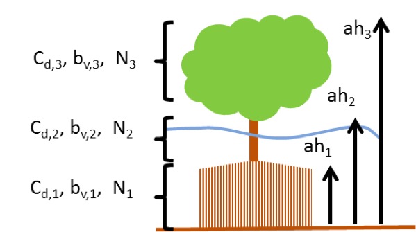
Fig. 11 Definition sketch of vegetation specification in XBeach (example for mangrove type vegetation schematized in three vertical sections).
Finally, the veggiemapfile indicates in what grid cell which vegetation species can be found. The format of this file is similar to the bathymetry files described in Grid and bathymetry, but the values are integers referring to a species where 1 refers to the first listed species, 2 to the second, et cetera. A zero indicates no vegetation at that particular location. The use of non-integer values in this file will result in an error.
In summary, the following files should be created when the effect of vegetation is modeled:
1 x Veggiemapfile: file similar to bathymetry file containing 0, 1 etc. (up to nveg)
1 x Veggiefile: list of file names of vegetation property files per species
nveg x vegetation property file(s): describing vegetation properties per species
Below the relevant keywords in the params.txt are given. In addition, the keyword vegetation should be set to 1.
parameter |
description |
default |
range |
units |
|---|---|---|---|---|
nveg |
Number of vegetation species |
-123 |
||
vegcanflo |
Include incanopy flow [1] or not [0] |
0 |
0 - 1 |
|
veggiefile |
Name of veggie species list file |
|||
veggiemapfile |
Name of veggie species map file |
|||
vegnonlin |
Include non-linear wave effect [1] or not [0] |
0 |
0 - 1 |
|
veguntow |
Include undertow in phase-averaged vegetati |
1 |
0 - 1 |
Porous in-canopy model input
The porous in-canopy model is aplied when the keyword porcanflow is set and the the physical process vegetation is included. A spatial varying canopy property can be used within the in-canopy model. This input is according to the vegetation input. Thus, the different coral types are described in the veggiefile and the location in the veggiemapfile. It is not possible to have different vertical sections in the canopy. Only the first vertical section is applied in the in-canopy model (nsec=1). The property file describes the canopy parameters ah, Cd, bv and N that represent the canopy height, drag coefficient, friction coefficient and the porosity (in percentage). The inertia coefficient is set by the keyword Cm and the permeability is set by the keyword Kp. An example of a property file is shown below for a coral,
coral.txt
nsec = 1
ah = 0.2
Cd = 15
bv = 0.1
N = 85
Discharge input
Discharge of water at the model boundaries or directly in the model domain is defined along specific grid sections. The keywords ndischarge and ntdischarge define the number of discharge sections and the length of the discharge time series respectively. The disch_loc_file keyword references a file that defines the discharge sections. Each line in this file corresponds to a grid section and each line contains four numbers being the start and end coordinates of the section. The file is formatted as follows, where ndisch refers to the keyword ndischarge:
disch_loc.txt
<x_start 1> <y_start 1> <x_end 1> <y_end 1>
<x_start 2> <y_start 2> <x_end 2> <y_end 2>
<x_start 3> <y_start 3> <x_end 3> <y_end 3>

...

<x_start ndisch> <y_start ndisch> <x_end ndisch> <y_end ndisch >
The world coordinates specified in this file must be chosen such that they are close to the desired grid cell borders, since the grid cell borders are eventually used as discharge section. Discharge sections can be located along grid cell borders that are either oriented cross-shore or alongshore, but not a combination of the two. In a regular grid this implies that either the start or end x-coordinates are equal, or the start and end y-coordinates are equal. Alternatively, both are equal. In this case a vertical discharge from above is assumed, rather than a horizontal discharge. Vertical discharges only add mass and no momentum to the water body.
The keyword disch_timeseries_file references a file defining the time series imposed on the discharge locations. The file lists the timings in the first column and a discharge value in \({\rm m}^{3}/{\rm s}\) for each discharge section as follows, where ntdisch refers to the keyword ntdischarge:
disch_timeseries.txt
<t 1> <Q 1,1> <Q 2,1> ... <Q ndisch,1>
<t 2> <Q 1,2> <Q 2,2> ... <Q ndisch,2>
<t 3> <Q 1,3> <Q 2,3> ... <Q ndisch,3>

...

<t ntdisch> <Q 1,ntdisch> <Q 2,ntdisch> ... <Q ndisch,ntdisch >
Discharges defined at the domain borders are positive in direction towards the domain (influx). Discharges defined in the domain itself are positive in direction of the positive x or y direction. Vertical discharges are positive into the domain (influx).

Fig. 12 Possible discharge orifices. A discharge orifice is defined as line in between two points (red). The resulting discharge orifice constitutes out of full abreast grid cells (green). The discharge direction is in positive grid direction (s or n), except at the domain border where the discharge is an influx in the domain (green arrows).
The table below gives an overview of all keywords related to discharges:
parameter |
description |
default |
range |
units |
|---|---|---|---|---|
disch_loc_file+ |
Name of discharge locations file |
<file> |
||
disch_timeseries_file+ |
Name of discharge timeseries file |
<file> |
||
ndischarge+ |
Number of discharge locations |
par%ndischarge |
0 - 100 |
|
ntdischarge+ |
Length of discharge time series |
par%ntdischarge |
0 - 100 |
Drifters input
Drifters can be deployed during the model simulation by specifying the number of drifters using the keyword ndrifter and the location, start and end time of the drifter deployment in a separate file referenced by the drifterfile keyword. The file format is as follows:
drifter.txt
<x 1> <y 1> <t_start 1> <t_end 1>
<x 2> <y 2> <t_start 2> <t_end 2>
<x 3> <y 3> <t_start 3> <t_end 3>

...

<x ndrifter> <y ndrifter> <t_start ndrifter> <t_end ndrifter>
The table below gives an overview of all keywords related to drifters:
parameter |
description |
default |
range |
units |
|---|---|---|---|---|
drifterfile |
Name of drifter data file |
<file> |
||
ndrifter |
Number of drifers |
par%ndrifter |
0 - 50 |
Ship-induced wave motions
Ship waves can be simulated by defining the ships’ geometries and trajectories in a collection of files. The user can define multiple ships. The number of ships is set by the keyword nship. In the file referenced by the keyword shipfile each ship is given a name. The properties of each ship are summarized in another textfile with the name of the ship (shipname.txt). This properties file defines the parameters for the discretization of the ships geometry. The ship grid is determined by the keywords dx, dy, nx, and ny, and the ship geometry itself is given in a separate file, referenced bythe keyword shipgeom. This file contains the ship draft per ship grid point, and should have a size of nx + 1 by ny + 1. The center of gravity of the ship is also defined in the ship properties file using the keywords xCG, yCG and zCG. The ships trajectory is defined in a file referenced from the ship properties file by the keyword shiptrack. Each row in this file contains a time, x- and y-coordinate indicating the ships position as function of time.
To avoid numerical problems, the full ship track should be within the model domain (i.e. a vessel cannot sail through the model boundary). Furthermore, it is advised to start the ship track with a very low velocity and gradually increase the sailing speed. When not taking into account such spin up period, the impact of the ship on the water level can be too abrupt, resulting in unrealistic wave patterns. In addition, it is advised to maintain a relatively deep edge of a few grid cells at both model boundaries (i.e. front and back side).
Another way to avoid numerical issues at the initialization of a ship simulation is to use the ‘flying’ option, which can be specified in the ship file (flying = 1). In case the option flying is enabled, also a z-coordinate is defined in the shiptrack-file indicating the vertical position of the ship. In this way, the vessel can ‘land’ on the water with its correct sailing speed, thereby avoiding unwanted disturbance to the water level. Also, the ship can ‘fly out’f the model domain before reaching the back boundary. By using this method the spin-up time can be reduced considerably and both inflow and outflow boundaries are unaffected by the ship
The two keywords compute_force and compute_motion enable the computation of forces on the ship and the ships motions due to wave forcing respectively; the latter has not been implemented yet. Forces on a ship in motion may be unreliable due to near-field effects; forces on a ship at rest are much more reliable. An example of ship definition files is:
shipfile.txt
containership.txt
oiltanker.txt
containership.txt
dx = 10
dy = 10
nx = 30
ny = 10
shipgeom = container_geom.dep
xCG = 120
yCG = 50
zCG = 30
shiptrack = container_track.txt
flying = 1
compute_force = 1
compute_motion = 1
pannamax_geom.txt
<z 0,0> <z 1,0> <z 2,0> <z 3,0> ... <z nx,0> <z nx+1,0>
<z 0,1> <z 1,1> <z 2,1> <z 3,1> ... <z nx,1> <z nx+1,1>

...

<z 0,ny> <z 1,ny> <z 2,ny> <z 3,ny> ... <z nx,ny> <z nx+1,ny>
<z 0,ny+1> <z 1,ny+1> <z 2,ny+1> <z 3,ny+1> ... <z nx,ny+1> <z nx+1,ny+1>
pannamax_track.txt
<t 1> <x 1> <y 1> <z 1>
<t 2> <x 2> <y 2> <z 2>
<t 3> <x 3> <y 3> <z 3>

...
oiltanker.txt
dx = 2
dy = 2
nx = 20
ny = 4
shipgeom = tanker_geom.dep
xCG = 20
yCG = 40
zCG = 1.5
shiptrack = tanker_track.txt
flying = 0
tanker_track.txt
<t 1> <x 1> <y 1>
<t 2> <x 2> <y 2>
<t 3> <x 3> <y 3>

...
parameter |
description |
default |
range |
units |
|---|---|---|---|---|
nship+ |
Number of ships |
-123 |
||
shipfile |
Name of ship data file |
<file> |
Output selection
Output selection determines what data computed by XBeach is written to a file in terms of location and time and in what format. The output types, output times and output formats supported by XBeach are explained in more detail in the following subsections. The table below gives an overview of all keywords related to model output:
parameter |
description |
default |
range |
units |
|---|---|---|---|---|
ncfilename+ |
Xbeach netcdf output file name |
<file> |
||
nglobalvar |
Number of global output variables (as specified by user) |
-1 |
-1 - 20 |
|
nmeanvar |
Number of mean, min, max, var output variables |
0 |
0 - 15 |
|
npoints |
Number of output point locations |
0 |
0 - 50 |
|
npointvar |
Number of point output variables |
0 |
0 - 50 |
|
nrugauge |
Number of output runup gauge locations |
0 |
0 - 50 |
|
nrugdepth+ |
Number of depths to compute runup in runup gauge |
1 |
1 - 10 |
|
outputformat+ |
Output file format |
fortran |
fortran, netcdf, debug |
|
outputprecision |
Switch between single and double precision output in netcdf |
double |
single, double |
|
timings+ |
Switch enable progress output to screen |
1 |
0 - 1 |
|
tintc+ |
Interval time of cross section output |
-123 |
s |
|
tintg |
Interval time of global output |
1.0 |
0.01 - par%tstop-par%tstart |
s |
tintm |
Interval time of mean, var, max, min output |
par%tstop-par%tstart |
1.0 - par%tstop-par%tstart |
s |
tintp |
Interval time of point and runup gauge output |
1.0 |
0.01 - par%tstop-par%tstart |
s |
tsglobal+ |
Name of file containing timings of global output |
|||
tsmean+ |
Name of file containing timings of mean, max, min and var output |
|||
tspoints+ |
Name of file containing timings of point output |
|||
tstart |
Start time of output, in morphological time |
0.0 |
0.0 - par%tstop |
s |
Output types
XBeach supports four different types of output: 1) instantaneous spatial output 2) time-averaged spatial output 3) fixed point output or 4) run-up gauge output. In principle any variable in XBeach can be outputted as long as it is part of the spaceparams structure defined in variables.f90 in the XBeach source code. An overview of all currently supported parameters in this file is presented in Table 25.
The amount of output variables used for each type is determined by the keywords nglobalvar, nmeanvar, npoints and nrugauge. Each of these keywords takes a number indicating the number of parameters or locations that should be written to file. If any of the keywords is set to zero, the output type is effectively disabled. If nglovalvar is set to -1 then a standard set of output variables is used, being H, zs, zs0, zb, hh, u, v, ue, ve, urms, Fc, Fy, ccg, ceqsg, ceqbg, Susg, Svsg, E, R, D and DR. If nglobalvar is not set it defaults to -1. The lines in the params.txt file immediately following these keywords determine what parameters or locations are used, as will be explained in more detail in the following subsections.
parameter |
description |
default |
range |
units |
|---|---|---|---|---|
As |
Asymmetry of short waves |
|||
BR |
Maximum wave surface slope used in roller dissipation formulation |
|||
Cdrag |
Vegetation drag coefficient |
|||
D |
Dissipation |
W/m2 |
||
D15 |
D15 grain diameters for all sediment classses |
m |
||
D50 |
D50 grain diameters for all sediment classses |
m |
||
D50top |
Friction coefficient flow |
|||
D90 |
D90 grain diameters for all sediment classses |
m |
||
D90top |
Friction coefficient flow |
|||
DR |
Roller energy dissipation |
W/m2 |
||
Dc |
Diffusion coefficient |
m2/s |
||
Df |
Dissipation rate due to bed friction |
W/m2 |
||
Dp |
Dissipation rate in the swash due to transformation of kinetic wave energy to potential wave energy |
W/m2 |
||
Dveg |
Dissipation due to short wave attenuation by vegetation |
W/m2 |
||
E |
Wave energy |
Nm/m2 |
||
Fvegu |
X-forcing due to long wave attenuation by vegetation |
N/m2 |
||
Fvegv |
Y-forcing due to long wave attenuation by vegetation |
N/m2 |
||
Fx |
Wave force, x-component |
N/m2 |
||
Fy |
Wave force, y-component |
N/m2 |
||
H |
Hrms wave height based on instantaneous wave energy |
m |
||
Hrunup |
Short wave height used in runup formulation |
m |
||
L1 |
Wave length (used in dispersion relation) |
m |
||
Qb |
Fraction breaking waves |
|||
R |
Roller energy |
Nm/m2 |
||
Sk |
Skewness of short waves |
|||
Subg |
Bed sediment transport for each sediment class (excluding pores), x-component |
m2/s |
||
Susg |
Suspended sediment transport for each sediment class (excluding pores), x-component |
m2/s |
||
Sutot |
Sediment transport integrated over bed load and suspended and for all sediment grains, x-component |
m2/s |
||
Svbg |
Bed sediment transport for each sediment class (excluding pores), y-component |
m2/s |
||
Svsg |
Suspended sediment transport for each sediment class (excluding pores), y-component |
m2/s |
||
Svtot |
Sediment transport integrated over bed load and suspended and for all sediment grains, y-component |
m2/s |
||
Sxx |
Radiation stress, x-component |
N/m |
||
Sxy |
Radiation stress, y-component |
N/m |
||
Syy |
Radiation stress, y-component |
N/m |
||
Tbore |
Wave period interval associated with breaking induced turbulence |
s |
||
Tsg |
Sediment response time for each sediment class |
s |
||
alfau |
Grid orientation at u-point |
rad |
||
alfav |
Grid orientation at v-point |
rad |
||
alfaz |
Grid orientation at z-point |
rad |
||
bedfriccoef |
Dimensional/dimensionless input bed friction coefficient; depends on value of parameter bedfriction |
|||
bi |
Incoming bound long wave |
m |
||
breaking |
Indicator whether cell has breaking nonh waves |
|||
bwalpha |
Beachwizard weighting factor |
|||
c |
Wave celerity |
m/s |
||
ca |
Reference concentration |
m3/m3 |
||
ccg |
Depth-averaged suspended concentration for each sediment fraction |
m3/m3 |
||
cctot |
Sediment concentration integrated over bed load and suspended and for all sediment grains |
m3/m3 |
||
ccz |
Concentration profile |
m3/m3 |
||
ceqbg |
Depth-averaged bed equilibrium concentration for each sediment class |
m3/m3 |
||
ceqsg |
Depth-averaged suspended equilibrium concentration for each sediment class |
m3/m3 |
||
cf |
Friction coefficient flow |
|||
cfu |
Friction coefficient flow in u-points |
|||
cfv |
Friction coefficient flow in v-points |
|||
cg |
Group velocity |
m/s |
||
cgx |
Group velocity, x-component |
m/s |
||
cgx_s |
Group velocity, x-component |
m/s |
||
cgy |
Group velocity, y-component |
m/s |
||
cgy_s |
Group velocity, y-component |
m/s |
||
cobs |
Beachwizard observed wave celerity |
m/s |
||
costh |
Cos of wave angles relative to grid direction |
|||
costh_s |
Cos of wave angles relative to grid direction |
|||
ctheta |
Wave celerity theta-direction (refraction) |
rad/s |
||
ctheta_s |
Wave celerity theta-direction (refraction) |
rad/s |
||
cx |
Wave celerity, x-component |
m/s |
||
cy |
Wave celerity, y-component |
m/s |
||
dU |
U-velocity difference between two vertical layers (reduced 2-layer non-hydrostatic model) |
m2/s2 |
||
dUi |
Velocity difference at boundary due to (short) waves |
m/s |
||
dV |
V-velocity difference between two vertical layers (reduced 2-layer non-hydrostatic model) |
m2/s2 |
||
dassim |
Beachwizard depth change |
m |
||
dcbdx |
Bed concentration gradient x-dir. |
kg/m3/m |
||
dcbdy |
Bed concentration gradient y-dir. |
kg/m3/m |
||
dcmdo |
Beachwizard computed minus observed dissipation |
W/m2 |
||
dcsdx |
Suspended concentration gradient x-dir. |
kg/m3/m |
||
dcsdy |
Suspended concentration gradient y-dir. |
kg/m3/m |
||
depo_ex |
Explicit bed deposition rate per fraction |
m/s |
||
depo_im |
Implicit bed deposition rate per fraction |
m/s |
||
dinfil |
Infiltration layer depth used in quasi-vertical flow model for groundwater |
m |
||
dnc |
Grid distance in n-direction, centered around c-point |
m |
||
dnu |
Grid distance in n-direction, centered around u-point |
m |
||
dnv |
Grid distance in n-direction, centered around v-point |
m |
||
dnz |
Grid distance in n-direction, centered around z-point (=eta-point) |
m |
||
dobs |
Beachwizard observed dissipation |
W/m2 |
||
dsc |
Grid distance in s-direction, centered around c-point |
m |
||
dsdnui |
Inverse of grid cell surface, centered around u-point |
1/m2 |
||
dsdnvi |
Inverse of grid cell surface, centered around v-point |
1/m2 |
||
dsdnzi |
Inverse of grid cell surface, centered around z-point |
1/m2 |
||
dsu |
Grid distance in s-direction, centered around u-point |
m |
||
dsv |
Grid distance in s-direction, centered around v-point |
m |
||
dsz |
Grid distance in s-direction, centered around z-point (=eta-point) |
m |
||
dzav |
Total bed level change due to avalanching |
m |
||
dzbdt |
Rate of change bed level |
m/s |
||
dzbdx |
Bed level gradient in x-direction |
|||
dzbdy |
Bed level gradient in y-direction |
|||
dzbed |
No description |
|||
dzbnow |
Bed level change in current time step |
m |
||
dzs0dn |
Alongshore water level gradient due to tide alone |
|||
dzsdt |
Rate of change water level |
m/s |
||
dzsdx |
Water surface gradient in x-direction |
m/s |
||
dzsdy |
Water surface gradient in y-direction |
m/s |
||
ee |
Directionally distributed wave energy |
J/m2/rad |
||
ee_s |
Directionally distributed wave energy |
J/m2/rad |
||
ero |
Bed erosion rate per fraction |
m/s |
||
fw |
Wave friction coefficient |
|||
gw0back |
Boundary condition back boundary for groundwater head |
m |
||
gwbottom |
Level of the bottom of the aquifer |
m |
||
gwcurv |
Curvature coefficient of groundwater head function |
|||
gwhead |
Groundwater head (differs from gwlevel) |
m |
||
gwheadb |
Groundwater head at bottom (differs from gwlevel) |
m |
||
gwheight |
Vertical size of aquifer through which groundwater can flow |
m |
||
gwlevel |
Groundwater table (min(zb,gwhead)) |
m |
||
gwqx |
Groundwater discharge in x-direction |
m/s |
||
gwqy |
Groundwater discharge in y-direction |
m/s |
||
gwu |
Groundwater flow in x-direction |
m/s |
||
gwv |
Groundwater flow in y-direction |
m/s |
||
gww |
Groundwater flow in z-direction (interaction between surface and ground water) |
m/s |
||
hh |
Water depth |
m |
||
hhw |
Water depth used in all wave computations, includes h*par%delta |
m |
||
hhwcins |
Water depth used in wave instationary computation in case of wci |
m |
||
hhws |
Water depth used in wave stationary computation (and single_dir wave directions) |
m |
||
hold |
Water depth previous time step |
m |
||
hu |
Water depth in u-points |
m |
||
hum |
Water depth in u-points |
m |
||
hv |
Water depth in v-points |
m |
||
hvm |
Water depth in v-points |
m |
||
idrift |
Drifter x-coordinate in grid space |
|||
infil |
Rate of exchange of water between surface and groundwater (positive from sea to groundwater) |
m/s |
||
istruct |
Location of revetments toe |
|||
iwl |
Location of water line (including long wave runup) |
|||
jdrift |
Drifter y-coordinate in grid space |
|||
k |
Wave number |
rad/m |
||
kb |
Near bed turbulence intensity due to depth induces breaking |
m2/s2 |
||
kturb |
Depth averaged turbulence intensity due to long wave breaking |
m2/s2 |
||
maxzs |
Maximum elevation in simulation |
m |
||
minzs |
Minimum elevation in simulation |
m |
||
n |
Ratio group velocity/wave celerity |
|||
nd |
Number of bed layers (can be different for each computational cell) |
|||
ndist |
Cum. distance from right boundary along n-direction |
m |
||
nuh |
Horizontal viscosity coefficient |
m2/s |
||
nutz |
Turbulence viscosity |
|||
pbbed |
No description |
|||
pdisch |
Discharge locations |
|||
ph |
Pressure head due to ship |
m |
||
pntdisch |
Point discharge locations (no momentum) |
|||
pres |
Normalized dynamic pressure |
m2/s2 |
||
qdisch |
Discharges |
m2/s |
||
qx |
Discharge in u-points, x-component |
m2/s |
||
qy |
Discharge in u-points, y-component |
m2/s |
||
refA |
Reference level |
m |
||
rolthick |
Long wave roller thickness |
m |
||
rr |
Directionally distributed roller energy |
J/m2/rad |
||
runup |
Short wave runup height |
m |
||
sdist |
Cum. distance from offshore boundary along s-direction |
m |
||
sedcal |
Equilibrium sediment concentartion factor for each sediment class |
|||
sedero |
Cum. sedimentation/erosion |
m |
||
setbathy |
Prescribed bed levels |
m |
||
shipFx |
Force on ship in x-direction |
N |
||
shipFy |
Force on ship in y-direction |
N |
||
shipFz |
Force on ship in z-direction |
N |
||
shipMx |
Moment on ship around x-axis |
Nm |
||
shipMy |
Moment on ship around y-axis |
Nm |
||
shipMz |
Moment on ship around z-axis |
Nm |
||
shipchi |
Turning angle arround y-axis |
deg |
||
shipphi |
Turning angle arround x-axis |
deg |
||
shippsi |
Turning angle arround z-axis |
deg |
||
shipxCG |
X-coordinate of ship center of gravity |
m |
||
shipyCG |
Y-coordinate of ship center of gravity |
m |
||
shipzCG |
Z-coordinate of ship center of gravity |
m |
||
shobs |
Beachwizard observed shoreline |
m |
||
sig2prior |
Beachwizard prior std squared |
m2 |
||
sigm |
Mean frequency |
rad/s |
||
sigt |
Relative frequency |
rad/s |
||
sigz |
Vertical distribution of sigma layers q3d |
|||
sinth |
Sin of wave angles relative to grid direction |
|||
sinth_s |
Sin of wave angles relative to grid direction |
|||
strucslope |
Slope of structure |
|||
structdepth |
Depth of structure in relation to instantaneous bed level |
m |
||
taubx |
Bed shear stress, x-component |
N/m2 |
||
taubx_add |
Additional bed shear stress due to boundary layer effects, x-component |
N/m2 |
||
tauby |
Bed shear stress, y-component |
N/m2 |
||
tauby_add |
Additional bed shear stress due to boundary layer effects, y-component |
N/m2 |
||
tdisch |
Discharge time series |
|||
tdriftb |
Drifter release time |
s |
||
tdrifte |
Drifter retrieval time |
s |
||
thet |
Wave angles |
rad |
||
thet_s |
Wave angles |
rad |
||
theta |
Wave angles directional distribution w.r.t. comp. x-axis |
rad |
||
theta_s |
Wave angles directional distribution w.r.t. comp. x-axis |
rad |
||
thetamean |
Mean wave angle |
rad |
||
tideinpt |
Input time of input tidal signal |
s |
||
tideinpz |
Input tidal signal |
m |
||
tsetbathy |
Points in time of prescibed bed levels |
s |
||
u |
Glm velocity in cell centre, x-component |
m/s |
||
ua |
Time averaged flow velocity due to wave assymetry |
m/s |
||
ucrcal |
Calibration factor for u critical for each sediment class |
|||
ududx |
Advection |
m2/s2 |
||
udvdx |
Advection |
m2/s2 |
||
ue |
Eulerian velocity in cell centre, x-component |
m/s |
||
ue_sed |
Advection velocity sediment in cell centre, x-component |
m/s |
||
ueu |
Eulerian velocity in u-points, x-component |
m/s |
||
ui |
Incident bound wave velocity in, x-component |
m/s |
||
umean |
Longterm mean velocity at bnds in u-points, x-component |
m/s |
||
umwci |
Velocity (time-averaged) for wci, x-component |
m/s |
||
ur |
Reflected velocity at bnds in u-points |
m/s |
||
urepb |
Representative flow velocity for sediment advection and diffusion, x-component |
m/s |
||
ureps |
Representative flow velocity for sediment advection and diffusion, x-component |
m/s |
||
urms |
Orbital velocity |
m/s |
||
usd |
Return flow due to roller after breaker delay |
m/s |
||
ust |
Stokes drift |
m/s |
||
ustr |
Return flow due to roller |
m/s |
||
ustz |
Stokes velocity (q3d) |
|||
uu |
Glm velocity in u-points, x-component |
m/s |
||
uv |
Glm velocity in v-points, x-component |
m/s |
||
uwcins |
U-velocity used in wave stationary computation in case of wci |
m/s |
||
uwf |
Stokes drift, x-component |
m/s |
||
uws |
U-velocity used in wave stationary computation (and single_dir wave directions) |
m/s |
||
uz |
Velocity (q3d) ksi-comp |
|||
v |
Glm velocity in cell centre, y-component |
m/s |
||
vdudy |
Advection |
m2/s2 |
||
vdvdy |
Advection |
m2/s2 |
||
ve |
Eulerian velocity in cell centre, y-component |
m/s |
||
ve_sed |
Advection velocity sediment in cell centre, y-component |
m/s |
||
vegtype |
Vegetation type index |
|||
vev |
Eulerian velocity in u-points, y-component |
m/s |
||
vi |
Incident bound wave velocity in, y-component |
m/s |
||
viscu |
Viscosity |
m2/s2 |
||
viscv |
Viscosity |
m2/s2 |
||
vmag |
Velocity magnitude in cell centre |
m/s |
||
vmageu |
Eulerian velocity magnitude u-points |
m/s |
||
vmagev |
Eulerian velocity magnitude v-points |
m/s |
||
vmagu |
Glm velocity magnitude u-points |
m/s |
||
vmagv |
Glm velocity magnitude v-points |
m/s |
||
vmean |
Longterm mean velocity at bnds in u-points, y-component |
m/s |
||
vmwci |
Velocity (time-averaged) for wci, y-component |
m/s |
||
vrepb |
Representative flow velocity for sediment advection and diffusion, y-component |
m/s |
||
vreps |
Representative flow velocity for sediment advection and diffusion, y-component |
m/s |
||
vu |
Glm velocity in u-points, y-component |
m/s |
||
vv |
Glm velocity in v-points, y-component |
m/s |
||
vwcins |
V-velocity used in wave stationary computation in case of wci |
m/s |
||
vwf |
Stokes drift, y-component |
m/s |
||
vws |
V-velocity used in wave stationary computation (and single_dir wave directions) |
m/s |
||
vz |
Velocity (q3d) eta-comp |
|||
wb |
Vertical velocity at the bottom |
m/s |
||
wete |
Mask wet/dry wave-points |
|||
wetu |
Mask wet/dry u-points |
|||
wetv |
Mask wet/dry v-points |
|||
wetz |
Mask wet/dry eta-points |
|||
wi |
Vertical velocity at boundary due to (short) waves |
m/s |
||
winddirts |
Input wind direction |
deg_nautical |
||
windinpt |
Input time of input wind signal |
s |
||
windnv |
Wind velocity in n direction in v point at current time step |
m/s |
||
windsu |
Wind velocity in s direction in u point at current time step |
m/s |
||
windvelts |
Input wind velocity |
m/s |
||
windxts |
Time series of input wind velocity (not s direction), x-component |
m/s |
||
windyts |
Time series of input wind velocity (not n direction), y-component |
m/s |
||
wm |
Mean abs frequency |
rad/s |
||
ws |
Vertical velocity at the free surface |
m/s |
||
wscrit |
Critial vertical velocity at the free surface for breaking |
m/s |
||
x |
X-coord. original cmp. grid |
m |
||
xHrunup |
Location at which short wave height for runup is taken |
m |
||
xu |
X-coord. comp. grid u-points |
m |
||
xv |
X-coord. comp. grid v-points |
m |
||
xyzs01 |
Global xy coordinates of corner (x=1,y=1) |
|||
xyzs02 |
Global xy coordinates of corner (x=1,y=n) |
|||
xyzs03 |
Global xy coordinates of corner (x=n,y=n) |
|||
xyzs04 |
Global xy coordinates of corner (x=n,y=1) |
|||
xz |
X-coord. comp. grid (positive shoreward, perp. to coastline) |
m |
||
y |
Y-coord. original comp. grid |
m |
||
yu |
Y-coord. comp. grid u-points |
m |
||
yv |
Y-coord. comp. grid v-points |
m |
||
yz |
Y-coord. comp. grid |
m |
||
z0bed |
No description |
|||
zb |
Bed level |
m |
||
zb0 |
Initial bed level |
m |
||
zbobs |
Beachwizard observed depth |
m |
||
zi |
Surface elevation at boundary due to (short) waves |
m |
||
zs |
Water level |
m |
||
zs0 |
Water level due to tide alone |
m |
||
zs0fac |
Relative weight of offshore boundary and bay boundary for each grid point is stored in zs0fac |
|||
zs1 |
Water level minus tide |
m |
||
zswci |
Waterlevel (time-averaged) for wci |
m |
Instantaneous spatial output
Instantaneous spatial output describes the instantaneous state of variables across the entire model domain at various points in time. To make use of this option the user must specify the number of output variables required using the nglobalvar keyword in params.txt, immediately followed by the names of the requested variables on a separate line each. The output of three instantaneous grids can look as follows:
params.txt
nglobalvar = 3
zs
zb
H
Time-averaged spatial output
Time-averaged spatial output describes the time-averaged state of variables across the entire model domain at various points in time. The user can define the averaging period in params.txt. To make use of this option the user must specify the number of output variables required using the nmeanvar keyword in params.txt, immediately followed by the names of the requested variables on a separate line each. The output of two time-averaged grids may look as follows:
params.txt
nmeanvar = 2
u
v
Fixed point output
Fixed point output allows the user to select one or more locations for which a time series of data is stored. This output describes a time-series of one or more variables at one point in the model domain. To make use of this option, the user must specify the number of output locations using the npoints keyword in params.txt, immediately followed by one line per output location describing the location coordinates given as the x-coordinate and y-coordinate and in world coordinates. XBeach will link the output location to the nearest computational point.
The user can specify the number and selection of output variables for all points (and run-up gauges, discussed in the following section) using the npointvar keyword in params.txt to specify the number of output variables, immediately followed by the names of the requested variables on a separate line each.
Fixed point output significantly reduces the amount of data written to file in each time step and is therefore particularly suitable for high temporal resolution output.
An example with two output locations is given below. The first point is located on the offshore boundary (x = 0.0) and somewhere in the middle of the model domain in y-direction (y = 800.0). The second point is located on the lateral boundary (y = 1600.0) and somewhere in the middle of the domain in x-direction (x = 2000.0). Both locations have four output variables: H, zs, zb and D.
params.txt
npoints = 2
0. 800.
2000. 1600.
npointvar = 4
H
zs
zb
D
Run-up gauge output
Run-up gauge output describes a time-series of a number of variables at the (moving) waterline. In this case XBeach scans in an x-directional transect defined by the user for the location of the waterline. Output information is recorded for this moving point. This is particularly useful to keep track of run-up levels in cross-shore transects.
The definition of run-up gauges is similar to the definition of fixed point output. The user needs to specify the number of run-up gauges using the nrugauge keyword in params.txt, immediately followed by one line per run-up gauge location describing the coordinates of the initial location of the run-up gauge. XBeach will subsequently link the initial run-up gauge location to the nearest computational cross-shore transect rather than just the nearest computational point.
Run-up gauges share their selection of output variables with regular point output. However, in the case of run-up gauges, XBeach will automatically also include the variables xw, yw and zs to the point output variables, if these variables were not specified using the npointvar keyword in params.txt. Note that the user should refer to the pointvars.idx output file to check order of output variables for points and run-up gauges.
An example of a run-up gauge input is given below. The run-up gauge is initially located on the offshore boundary (x = 0.0) and somewhere in the middle of the model domain in y-direction (y = 800.0). The run-up gauge will display standard output variables (xw, yw and zs, as well as any output variables specified by the npointvar keyword).
params.txt
nrugauge = 1
0. 800.
Output times
The user may determine the output times for regular spatial output variables, time averaged spatial variables and point location variables individually. Run-up gauge output and fixed point output are given at the same moments in time. For all three types of output the user may choose to either state a fixed interval time at which output is given or supply an external file containing times at which output should be given or a combination of both.
Output at fixed intervals
The user should define a point in time after the start of the simulation at which the first output is generated for fixed interval output. The user can do this by using the tstart keyword in params.txt. All output that is being generated at fixed intervals uses tstart as their base. The interval for instantaneous spatial output is given by the tintg keyword. The keywords for the interval of time-averaged spatial output and point output are tintm and tintp respectively, where tintp is used both for fixed point and run-up gauge output. Note that tintg, tintm and tintp supersede the older tint parameter that is valid for all types of output. The default value of tintg is one second. If tintp or tintm is not stated, but output is declared (npoints, nrugauge or nmeanvar is stated larger than zero), XBeach assumes the same output interval as tintg. An example of the definition of fixed intervals is given below.
params.txt
tstart = 100.
tintg = 100.
tintp = 2.
tintm = 3600.
In the case of instantaneous spatial output and point output, the first output is given at tstart. In the case of time-averaged spatial variables, the first output is given at tstart+tintm. This output represents the average condition over the interval between tstart and tstart+tintm.
Output times defined by external file
The user is given the option to have output at a set of points in time that are not separated by regular intervals. In this case the user must supply an additional file for each output type. The user specifies the name of the output time series file for instantaneous spatial output using the tsglobal keyword. The keywords for time series files for time-averaged spatial output and point output are tsmean and tspoint respectively, where tspoint is again used for both fixed point and run-up gauge output. All time series files must contain on the first line the number of output times followed by every output time on a new line. An example of such irregular output time definition is given below.
params.txt
tsglobal= time_series1.txt
tspoints = time_series2.txt
tsmean= time_series3.txt
time_series1.txt
18
0.05
0.15
0.2
0.8
12.0
12.5
19.124
30.
60.
90.
120.
150.
160.
170.
177.
178.
179.
180.
In the case of instantaneous spatial output and point output, the first output is given at the first stated point in time. In the case of time-averaged spatial variables, the first output is given at the second stated point in time. This output represents the average condition over the interval between first and second stated point in time. Subsequent averaging is done over every interval.
Combinations of fixed internal and external files
The user is allowed to define certain types of output using fixed intervals and others using external files. The use of an external file supersedes the use of fixed intervals. Note that tstart will only apply to output of fixed interval type. An example of mixing fixed and varying output time intervals is given below.
param.txt
tstart = 100.
tintg = 100.
tspoints = time_series2.txt
tintm = 3600.
Output format
XBeach supports two types of output: 1) Fortran binary and 2) netCDF. The output format used is determined by the keyword outputformat. The use of netCDF output is more convenient since all output (and input) is stored in a single, easy accessible file. Also the netCDF file format is compatible with many programming languages (e.g. Matlab, Python) as well as many visualization tools (e.g. QuickPlot, Morphan). It should be noted that the support for output types in netCDF could be limited for recent functionalities of the XBeach model.
Fortran binary
Output files in Fortran binary format are bare matrix dumps of XBeach’ computational matrices. At each output time, one such matrix block is added to the output file. These files can generally be read by binary read functions, like fread in Matlab and the struct package in Python.
Output files written in Fortran binary format are given the name < variable >.dat, for example zs.dat, for instantaneous spatial output. The only exception is that files containing information about the wave height of the short waves are called hrms.dat instead of H.dat to maintain backward compatibility. Time-averaged spatial output is stored similarly, but the file names have a suffix indicating the type of averaging < variable >_mean.dat. For time-averaged spatial output also the variance, minimum and maximum values are stored using the suffixes _var, _min and _max respectively.
All data corresponding to fixed point locations will be stored in files called point< NNN >.dat. < NNN > represents a number between 001 and 999 corresponding to the order in which the points are declared in params.txt. The data files are plain text and contain one row for each output time step. The first position on each row is the time at which the output is given. The subsequent positions in the row are the instantaneous values of the variables at the given point. The order of the variables is equal to the order in which they are defined for that point in params.txt. Data corresponding to run-up gauge locations are stored in the same format as fixed point output, but the files are named rugau< NNN >.dat.
An extra file called dims.dat is always written at the start of the simulation in Fortran binary output mode. This file contains the dimensions of the XBeach model. It simply states the following dimensions in order: nt (number of output time steps), nx (number of grid cells in x-direction), ny (number of grid cells in y-direction), ngd (number of sediment fractions), nd (number of bed layers), ntp (number of point output time steps), ntm (number of time-averaged output time steps). Subsequently, the irregular time series are stored, if applicable: tsglobal (irregular output times), tspoints (irregular point output times) and tsmean (irregular time-averaged output times). Similarly, a file xy.dat is written containing the x- and y- coordinates of the full computational grid.
netCDF
All data in netCDF output is stored in a single output file. By default this file is named xboutput.nc, but this name can be chosen freely using the keyword ncfilename. The netCDF file holds all output data, dimensions and input data in a single file. It should be noted that netCDF files can hold a multiple time axes. The temporal unit can be specified in the params.txt file using the keyword tunits. This unit does not affect calculations and is only used for output. An example of the layout of the netcdf file is given below:
xboutput.nc (structure only, no real contents)
netcdf xboutput {
   dimensions:
      x = 565 ;
      y = 101 ;
      wave_angle = 9 ;
      bed_layers = 3 ;
      sediment_classes = 1 ;
      inout = 2 ;
      globaltime = 2 ;
      tidetime = 435 ;
      tidecorners = 2 ;
      windtime = 2 ;
   variables:
      double x(x) ;
         x:units = 'm' ;
         x:long_name = 'local x coordinate' ;
      double y(y) ;
         y:units ='m' ;
         y:long_name = 'local y coordinate';
      double globaltime(globaltime) ;
         globaltime:units = 's' ;
      double H(globaltime, y, x) ;
         H:units = 'm' ;
         H:long_name = 'wave height' ;
      double zs(globaltime, y, x) ;
         zs:units = 'm' ;
         zs:long_name = 'water level' ;
      double zb(globaltime, y, x) ;
         zb:units = 'm' ;
         zb:long_name = 'bed level' ;
      double ue(globaltime, y, x) ;
         ue:units = 'm/s' ;
}
Time parameters
In all XBeach simulations the hydrodynamic simulation starts at time 0. Model output can be postponed until the time specified by the keyword tstart. The simulation stops at the time specified by tstop. The time step used in the hydrodynamic simulation is determined based on a given maximum Courant number using the keyword CFL. The table below gives an overview of all keywords related to time management:
parameter |
description |
default |
range |
units |
|---|---|---|---|---|
CFL |
Maximum courant-friedrichs-lewy number |
0.7 |
0.1 - 0.9 |
|
defuse |
Turn on timestep explosion prevention mechanism |
1 |
0 - 1 |
|
dtset |
Fixed timestep, overrides use of cfl |
0.0 |
0.001 - 100.0 |
|
maxdtfac |
Maximum increase/decrease in time stp in explosion prevention mechanism |
500.0 |
100.0 - 1000.0 |
|
tstop* |
Stop time of simulation, in morphological time |
2000.0 |
1.0 - 1000000.0 |
s |
tunits+ |
Time units in udunits format (seconds since 1970-01-01 00:00:00.00 +1:00) |
s |