XBeach Matlab Toolbox (tutorial)

Set-up model

XBeach is configured using a collection of files that hold information on the bathymertry, boundary conditions, model settings, etcetera. All files are plain text files that should be in a single directory, the model run directory. Running the XBeach executable in this directory, will make XBeach use those files and save the model output in the very same directory.

Using the Matlab Toolbox, setting up your model is made much easier. On this page we explain how to set-up a simple model using the Matlab Toolbox. The toolbox creates a bunch of files, which we will explain. Setting up a model manually, without the toolbox, implies creating these files in any other way of your preference. A collection of example models can be found in the Documentation section.

Generate model with xb_generate_model

Having started Matlab and incLuded the Matlab XBeach Toolbox to your path, you should be able to run the following command:

xbi = xb_generate_model;

When done, the xbo variable now contains a structure with a full XBeach model set-up. You can write the model to disk by running the following command:

xb_write_input('params.txt', xbi);

The file params.txt, which contains all model settings, is now written to your current directory along with several other files which are referred to from the params.txt file. The different files are listed below:

File	Description
params.txt	File with model settings. Each line containing an =-sign and not starting with a %-sign is interpreted as a model setting in the form “name = value”. This file is obligatory when running XBeach. It also refers to the other files.
bed.dep	File with bathymetry information. It simply contains the heights for all grid points. On row corresponds to one cross-shore transect. This file is obligatory when running XBeach.
x.grd	File with x-coordinates of the grid. This file is only used with a non-equidistant grid.
y.grd	File with y-coordinates of the grid. This file is only used with a non-equidistant two-dimensional grid.
jonswap.txt	File with boundary condition information. In this case the description of a JONSWAP spectrum. Severel flavours exist for this file. This one has a syntax similar to the params.txt file.

When we open the file params.txt with a text editor, we get the following content:

%%%%%%%%%%%%%%%%%%%%%%%%%%%%%%%%%%%%%%%%%%%%%%%%%%%%%%%%%%%%%%%%%%%%%%%%%%%%%%%%
%%% XBeach parameter settings input file                                     %%%
%%%                                                                          %%%
%%% date:     29-Jun-2016 07:40:37                                           %%%
%%% function: xb_write_params                                                %%%
%%%%%%%%%%%%%%%%%%%%%%%%%%%%%%%%%%%%%%%%%%%%%%%%%%%%%%%%%%%%%%%%%%%%%%%%%%%%%%%%

%%% Grid parameters %%%%%%%%%%%%%%%%%%%%%%%%%%%%%%%%%%%%%%%%%%%%%%%%%%%%%%%%%%%%

depfile   = bed.dep
posdwn    = 0
nx        = 580
ny        = 0
alfa      = 0
vardx     = 1
xfile     = x.grd
yfile     = y.grd
xori      = 0
yori      = 0
thetamin  = 225
thetamax  = 315
dtheta    = 90
thetanaut = 1

%%% Initial conditions %%%%%%%%%%%%%%%%%%%%%%%%%%%%%%%%%%%%%%%%%%%%%%%%%%%%%%%%%

zs0       = 5

%%% Model time %%%%%%%%%%%%%%%%%%%%%%%%%%%%%%%%%%%%%%%%%%%%%%%%%%%%%%%%%%%%%%%%%

tstop     = 2000

%%% Wave boundary condition parameters %%%%%%%%%%%%%%%%%%%%%%%%%%%%%%%%%%%%%%%%%

instat    = jons

%%% Wave-spectrum boundary condition parameters %%%%%%%%%%%%%%%%%%%%%%%%%%%%%%%%

bcfile    = jonswap.txt
rt        = 1800
dtbc      = 1

%%% Output variables %%%%%%%%%%%%%%%%%%%%%%%%%%%%%%%%%%%%%%%%%%%%%%%%%%%%%%%%%%%

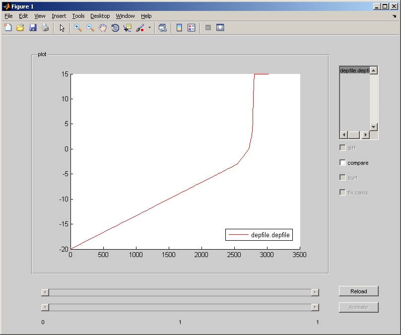
The files describe a simple one-dimensional model with a schematized dune profile (see Figure) and a statistically constant boundary conditions described by a JONSWAP spectrum with a significant wave height of 7.6m and a peak wave period of 12s.

Arguments of the xb_generate_model

Run model

You can run your model by simply executing the XBeach executable in the directory where you wrote your models settings to. This is the directory where the params.txt file is located.

If your created your model using the Matlab Toolbox, you can run the model from within Matlab. As shown in the previous step, you can store an entire XBeach model setup in a single Matlab variable. To run this model, simply use one of the following commands:

xbr = xb_run(xbi);
xbr = xb_run(xbi, 'binary', 'xbeach.exe', 'name', 'MyFirstXBeachModel');

When you use the first command, a directory with a unique name is created in your current working directory. The model setup is written to that directory, the latest XBeach executable is downloaded from this open-source software portal and the model is run. The function returns a structure with information on the run just started.

When you want to use another executable, you can define the executable using the binary option. Also, you can give the run a name, which is used as directory name as well. This is shown in the second command.

If you have a UNIX cluster available running Sun Grid Engine (SGE), you might be able to use the remote version of the run command. The cluster should be able by SSH. The command looks like this:

xbr = xb_run_remote( ...``
         'binary', 'xbeach', 'name', 'MyFirstXBeachModel', ...
         'ssh_host', 'h4', 'ssh_prompt', true);

Visualize results

Once your model finished running, it is time to have a look at the model output. Two types of output can be generated: Fortran and netCDF. The former type generates a series of DAT files as output, while the latter generates a single NC file with all data in it. The Matlab Toolbox supports both and there are no significant differences in the usage of the commands shown.

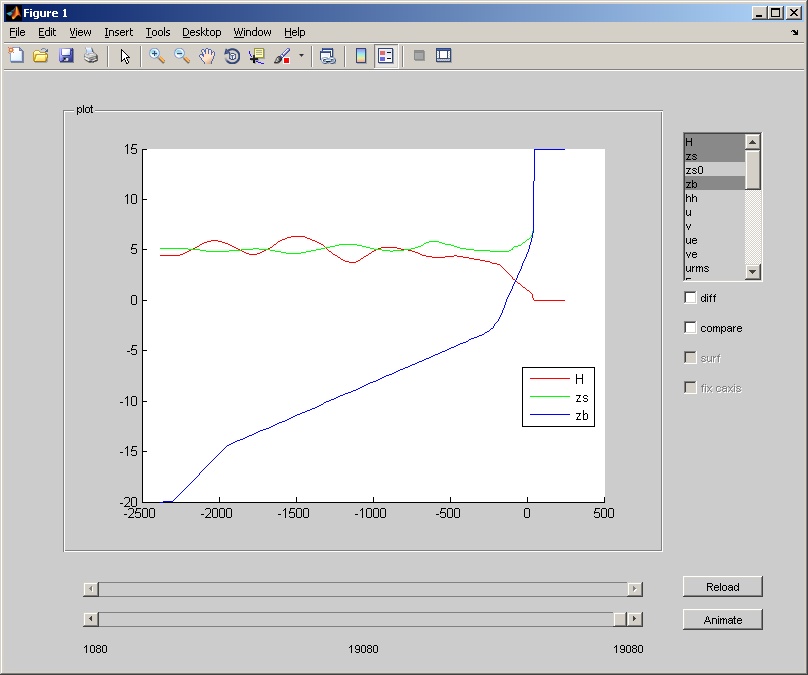
To have a quick view on your model output, use the xb_view command. This command works as well while the model is still running. Just run the command in the model directory, supply the model directory or supply the result structure from the xb_run command:

xb_view;
xb_view('MyFirstXBeachModel/');
xb_view(xbr);

The result will be somethink like this:

If you need to manipulate the output data or the visualization a bit more than the xb_view command offers, you will need to load the output data. The output is read using the xb_read_output command, which stores the data in an XBeach structure. The xs_peel command converts this structure to a regular structure with matrices with dimensions time, y and x. The dimensions itself are read by the xb_read_dims command. Try the following commands to figure out how it all works:

xbo = xb_read_output;
xbo = xb_read_output('MyFirstXBeachModel/');
xbo = xb_read_output(xbr);

xbo = xb_read_output(pwd, 'vars', 'H');
xbo = xb_read_output(pwd, 'vars', {'H' 'zb'});
xbo = xb_read_output(pwd, 'vars', {'H' 'zb'}, 'length', 1);
xbo = xb_read_output(pwd, 'vars', {'H' 'zb'}, 'length', [1 1 -1]);
xbo = xb_read_output(pwd, 'vars', {'H' 'zb'}, 'length', [1 1 -1], 'start', 100);
xbo = xb_read_output(pwd, 'vars', {'H' 'zb'}, 'length', [1 1 -1], 'start', [100 2 1]);
xbo = xb_read_output(pwd, 'vars', {'H' 'zb'}, 'length', [1 1 -1], 'start', [100 2 1], 'stride', [1 1 5]);
xbo = xb_read_output(pwd, 'vars', '*_mean');
xbp = xs_peel(xbo);
xs_peel(xbo);

xbd = xb_read_dims;
xbd = xb_read_dims('MyFirstXBeachModel/');
xbd = xb_peel(xbp.DIMS);

plot(xbd.x, squeeze(xbp(end,1,:)));

Analyze results

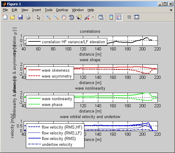
What we did so far is setting-up and running a simple model and visualizing the results. The visualization was limited to a plain representation of the model output. Often, it is necessary to obtain insight in the overall characteristics of the model results in wave propagation and erosion progression in terms of volumes or retreat distances. This section describes a few simple tools to extract these characteristics from the model output.

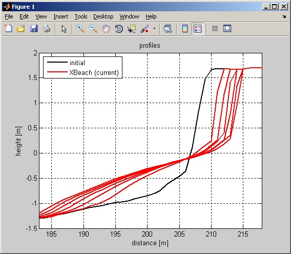
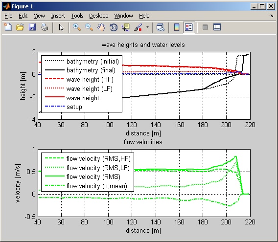
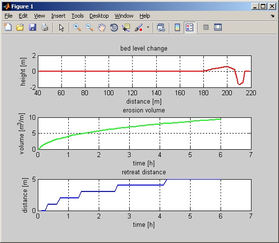
Analysis methods for the following aspects of dune and beach morphology are currently available:

Profiles

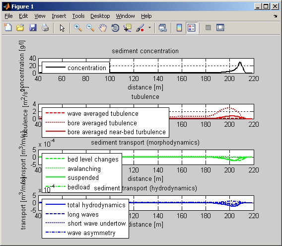
Hydrodynamics

Sediment transports

Morphodynamics

The following collection of commands and screenshots provide an overview of what is possible. Of course, you are encouraged to write your own analysis scripts and, if generally applicable, provide it to the community!

Profiles

xb_plot_profile(xbo);

Hydrodynamics

xbh = xb_get_hydro(xbo);
xb_plot_hydro(xbh);
xb_plot_hydro2(xbh);

Sediment transports

xbs = xb_get_sedtrans(xbo);
xb_plot_sedtrans(xbs);

Morphology

xbm = xb_get_morpho(xbo);
xb_plot_morpho(xbm);