Numerical implementation
Grid set-up
The new implementation utilizes a curvilinear, staggered grid where depths, water levels, wave action and sediment concentrations are given in the cell centers (denoted by subscript z) and velocities and sediment fluxes at the cell interfaces (denoted by subscript u or v). In Fig. 13 the z, u, v and c (corner) points with the same numbering are shown. The grid directions are named s and n; grid distances are denoted by \(\Delta s\)and \(\Delta n\), with subscripts referring to the point where they are defined. A finite-volume approach is utilized where mass, momentum and wave action are strictly conserved. In the middle panel of Fig. 13, the control volume for the mass balance is shown with the corresponding grid distances around the u- and v-points. The right panel explains the numbering of the fluxes Q and the volume V.
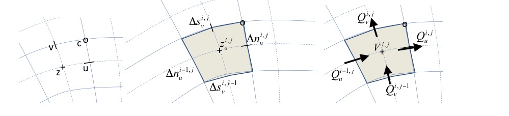
Fig. 13 Location of staggered grid points (left panel); definition of grid distances (middle) and terms in volume balance (right)
Wave action balance
Surfbeat solver
The time-varying wave action balance solved in XBeach is as follows:
Where \(E\) is the wave energy or wave action, \(C_g\) is the group velocity, \(C_{\vartheta}\)the refraction speed in theta-space and \(Sink\) refers to effects of wave breaking and bottom friction.
Again, the advection terms are the only ones affected by the curvilinear scheme so we will discuss their treatment in detail. The control volume is the same as for the mass balance. In equation (134) the procedure to compute the wave energy fluxes across the cell boundaries is outlined. All variables should also have an index \(itheta\) referring to the directional grid, but for brevity these are omitted here.
The component of the group velocity normal to the cell boundary, at the cell boundary, is interpolated from the two adjacent cell center points. Depending on the direction of this component, the wave energy at the cell boundary is computed using linear extrapolation based on the two upwind points, taking into account their grid distances. This second order upwind discretization preserves the propagation of wave groups with little numerical diffusion.
The other three fluxes are computed in a similar way; for brevity we will not present all formulations.
The time integration is explicit and the same as in the original implementation. The advection in u- and v-direction is computed simply by adding the four fluxes and dividing by the cell area. This procedure guarantees conservation of wave energy.
The procedure for the roller energy balance is identical to that for the wave energy balance and will not be repeated here.
Stationary solver
In the stationary solver the wave energy and roller energy balances are solved line by line, from the seaward boundary landward. For each line the automatic timestep is computed and the quasi-time-dependent balance is solved until convergence or the maximum number of iterations is reached, after which the solver moves to the next line.
The iteration is controlled by the parameters maxiter and maxerror.
Shallow water equations
Mass balance equation
The mass balance reads as follows:
This is discretized according to:
Here, \({A}_{z}\) is the area of the cell around the cell centre, \({z}_{s}\) is the surface elevation, \({u}_{u}\) is the u-velocity in the u-point, \({h}_{u}\) the water depth in the u-point and \({v}_{v}\) the v-velocity in the v-point. The indices \(i,j\) refer to the grid number in u resp. v direction; the index \(n\) refers to the time step.
Momentum balance equation
Second, we will outline the derivation of the u-momentum balance. The control volume is given in Fig. 14. It is centeredaround the u-point. We now consider the rate of change of the momentum in the local u-direction as follows:
where V is the cell volume, u the velocity in local grid direction, Q the fluxes,\(\rho\) the density, g acceleration of gravity, \(\tau_{b,u}, \tau_{b,u}, F_{u}\) the bed shear stress, wind shear stress and wave force in u-direction. We consider that the outgoing fluxes carry the velocity inside the cell, \(u\), and that \({u}_{in}\) is determined at each inflow boundary by interpolation, reconstructing the component in the same direction as \(u\).
The volume balance for the same volume reads:
By multiplying the volume balance by \(u\), subtracting it from the momentum balance and dividing the result by \(V\) we arrive at the following equation:
where \(A\) is the cell area and \({h}_{um}\) is the average depth of the cell around the u-point. The procedure for the second term (the others are straightforward) now boils down to integrating (only) the incoming fluxes over the interfaces and multiplying them with the difference between \(u\) in the cell and the component of velocity in the same direction at the upwind cell.
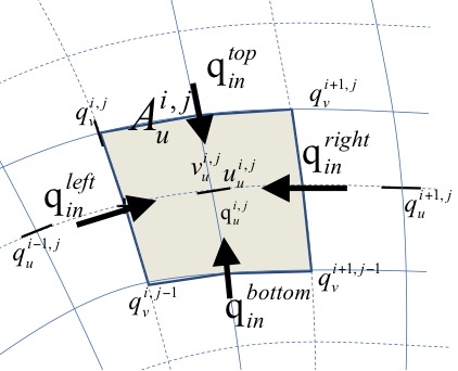
Fig. 14 Control volume u-momentum balance and definition of fluxes
In the following three quations the procedure for computing the u-momentum balance is outlined. The discharges in the u-points are computed by multiplying the velocity in the u- or v-point by the water depth at that point. These discharges are then interpolated to the borders of the control volume around the u-point. The difference \(\Delta \alpha\)in grid orientation between the incoming cell and the u-point is computed and used to compute the component of the incoming velocity in the local u-direction, from the left and right side of the control volume.
The same is done for the top and bottom of the control volume, based on the discharges in v-direction:
Finally, the advective term in the momentum balance is given as:
Time integration scheme
The time integration of the mass and momentum balance equations is combined in an explicit leap-frog scheme, as depicted in Fig. 15. The velocities are updated using the momentum balance, the water levels are updated using the mass balance. The water level gradients influence the momentum balance and the velocities and derived discharges affect the mass balance. Because of the leap-frog scheme these influences are always computed at the half time step level, which makes the scheme second order accurate.
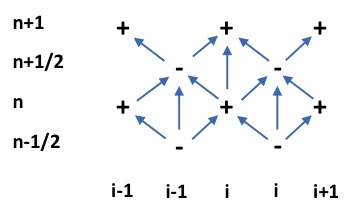
Fig. 15 Leap-frog time integration scheme
Using this straightforward finite volume approach, complicated transformations of the equations are avoided and the solution scheme remains transparent. It is also completely compatible with the original rectilinear implementation and is even slightly more efficient.
Groundwater flow
In order to solve the equations in xx, the spatial and temporal domain of the groundwater system is split into the same spatial grid and time steps as the XBeach surface water model it is coupled to. At each time step in the numerical model, the depth average groundwater head is calculated in the center of the groundwater cells, and the fluxes (specific discharge, submarine exchange, infiltration and exfiltration) are calculated on the cell interfaces
At the start of the time step, every cell is evaluated whether the groundwater and surface water are connected:
In equation (143) \(\varepsilon\) is a numerical smoothing constant used to deal with numerical round off errors near the bed (equal to the parameter dwetlayer in the case of hydrostatic groundwater flow, and to the parameter eps in the case of non-hydrostatic groundwater flow), and \(i\) and \(j\) represent cross-shore and longshore coordinates in the numerical solution grid, respectively. Infiltration is calculated in cells where the groundwater and surface water are not connected and there exists surface water. As shown in equation (81) the infiltration rate is a function of the thickness of the wetting front, which is zero at the start of infiltration, and increases as a function of the infiltration rate. The equations for the infiltration rate and the thickness of the wetting front are approximated by first-order schemes, in which the wetting front is updated using a backward-Euler scheme, which ensures numerical stability:
In the pressure term \({p}_{lpf}\) is the surface water pressure at the bed, which in the case of non-hydrostatic surface water flow is high-pass filtered at \(4/{T}_{rep}\), the superscript \(n\) corresponds to the time step number and \(\Delta t\) is the size of the time step. The infiltration rate in the coupled relationship can be solved through substitution:
At the end of infiltration, i.e. when the groundwater and surface water become connected or there is no surface water left, the wetting front thickness is reset to zero. If the infiltration rate exceeds the Reynolds number for the start of turbulence, the local hydraulic conductivity is updated using the local Reynolds number:
XBeach iterates until a minimum threshold difference between iterations is found for and . Infiltration in one time step is limited to the amount of surface water available in the cell and to the amount of water required to raise the groundwater level to the level of the bed:
If during infiltration the groundwater level reaches the bed level, the fraction of the time step required to do so is estimated (x) and the remaining fraction is used in the submarine exchange.
Exfiltration is calculated in cells where the groundwater and surface water are not connected and the groundwater level exceeds the bed level:
Horizontal infiltration and exfiltration (keyword: gwhorinfil = 1) is computed across the numerical vertical interface between the groundwater domain and the surface water domain in adjoining cells. The direction of exchange is determined by the head gradient, and the bed level slope direction:
After infiltration and exfiltration have been calculated, the groundwater level and surface water level are updated:
All updated cells are subsequently re-evaluated on whether the surface water and groundwater are connected or unconnected
The cell height at the center of the groundwater cells (\(\Delta z_{H,i,j}\)) is calculated from the groundwater level and the bottom of the aquifer in the center of the cell, whereas the cell heights at the horizontal cell interfaces are calculated using an upwind procedure:
In \({z}_{aquifer}\) is the level of the bottom of the aquifer. As described in Sediment transport, the head applied on the top boundary of the groundwater domain (\({H}_{bc}\)) depends on whether the groundwater and surface water are connected or unconnected:
In the parameter \(\kappa_{r}\) is the relative numerical ‘connectedness’ of the groundwater and surface water head, determined by linear interpolation across the numerical smoothing constant \(\varepsilon\).
In the case of hydrostatic groundwater flow, the groundwater head in each cell is set equal to the head applied on the top boundary of the groundwater domain (\({H}_{bc}\)) and the horizontal groundwater flux is computed from the groundwater head gradient:
In the superscripts \(x\) and \(y\) refer to the components of the variable in the cross-shore and longshore direction, respectively, and the subscripts \(u\) and \(v\) refer to variables approximated at the horizontal cell interfaces in the cross-shore and longshore direction, respectively.
In the case of non-hydrostatic groundwater flow, the horizontal specific discharge on each cell interface can be found through an approximation of the non-hydrostatic groundwater head gradient:
In the subscript \(H\) refers to variables approximated at the cell centers. The hydraulic conductivity may be different at each cell interface and is therefore computed at every interface where every K is calculated separately.
Continuity in the groundwater cell is found following:
In the variable \({q}^{z}\) refers to the vertical groundwater discharge (e.g., submarine exchange if connected to the surface water, or groundwater level fluctuations if the groundwater is not connected to the surface water).
In the case of hydrostatic groundwater flow, the variable \({q}^{z}\) can be solved through the known variables \({q}^{x}\) and \({q}^{y}\). However, in the case of non-hydrostatic groundwater flow, all variables in contain an unknown value for the groundwater pressure head, described in terms of a known head at the surface of the groundwater (\({H}_{bc}\)) and the unknown curvature of the vertical groundwater head function (\(\beta\)). Since water is incompressible, the groundwater pressure must be solved for all cells simultaneously using matrix algebra:
In A is a matrix containing coefficients for the horizontal and vertical specific discharge, x is a vector containing the unknown groundwater head curvature, and b contains the known forcing terms. For a one dimensional cross-shore case, A is reduced to a tridiagonal matrix. The vector of known forcing consists of the numerical gradients in the contribution of the head applied on the top boundary of the groundwater domain to the horizontal specific discharge.
In the one dimensional case, the solution to the tridiagonal matrix A can be computed using the efficient Thomas algorithm ([Thomas, 1949]). In the two dimensional case, matrix A contains two additional diagonals that are not placed along the main diagonal, and vector b contains additional forcing terms from the alongshore contribution. The solution to the two dimensional case requires a more complex and less computationally efficient matrix solver. In this case the Strongly Implicit Procedure ([Stone, 1968]) is used in a manner similar to [Zijlema et al., 2011]. The horizontal and vertical groundwater fluxes are calculated using the solution of x plus and .
Since in both hydrostatic and non-hydrostatic groundwater flow some local velocities may exceed the critical Reynolds number for the start of turbulence (\({Re}_{crit}\)), the turbulent hydraulic conductivity (\(K\)) is updated using the local Reynolds number. The solution to and the update of the turbulent hydraulic conductivity are iterated until a minimum threshold difference between iterations is found. Note that this approach is only used is the turbulent groundwater model is selected (keyword: gwscheme = turbulent).
The (iterated) solution for the specific vertical discharge is used to update the groundwater level and surface water level:
If the groundwater and surface water are connected, and the submarine exchange from the surface water to the groundwater estimated in is greater than the amount of surface water available in the cell, continuity is enforced by lowering the groundwater level to compensate for the lack of permeating water:
Sediment transport
The advection-diffusion equation for suspended sediment is the basis for the sediment transport computations in XBeach. The partial differential equation to solve is:
Here \(c\) is the depth-averaged concentration, \({c}_{eq}\) the equilibrium concentration, \(Ts\) a typical timescale proportional to water depth divided by fall velocity. As is often done to increase robustness, we treat the erosion term explicitly but take an implicit scheme for the sedimentation term:
This can be rewritten as:
The sediment transport gradient is discretized in a similar way as the mass balance:
The sediment transports in the u- points contain an advective term, a diffusive term and a bed slope term:
Here \({u}_{rep,s}\) is a representative velocity for suspended transport, which contains contributions due to return flow, wave skewness and wave asymmetry; \({D}_{c}\) is a horizontal diffusion coefficient and \({f}_{slope}\) a coefficient. In discretized form the expression for the suspended transport in the u-point is:
The concentrations in the u-points are computed with a \(\theta\) -method, where \(\theta=1\) means a fully upwind approximation, and \(\theta=0.5\) a central scheme. In practice, we mostly use the upwind approximation for its robustness.
The erosion and deposition terms, which may also be used in the bed updating, are finally computed from:
The evaluation of the bedload transport takes place in the same way as in the previous versions of XBeach, except for the fact that the directions are taken in local grid direction, and will not be repeated here.
Bottom updating schemes
Two alternative formulations are available for the bed updating: one where the bottom changes are computed based on the gradients of suspended and bed load transport, equation (168) , and one where the changes due to suspended transport are accounted for through the erosion and deposition terms, equation (169).
In both cases \(MF\) is the morphological factor used to accelerate morphological changes. In the first case, the sediment in the bottom is conserved in all cases, but changes in the amount of sediment in the water are not considered; one can also say that the sediment in suspension is added to the bottom sediment. In the second case, the storage of sediment in the water is accounted for, but will be distorted in cases of high \(MF\). Since under most circumstances the real effect of the storage in the water phase is small we prefer the first formulation which guarantees mass conservation in the bottom. Both formulations are calculated using an explicit scheme:
Avalanching
XBeach implements avalanching as described in section Avalanching. It first calculates bed level change due to avalanching in the cross-shore dimension. It then calculates the slopes in alongshore direction and bottom change due to avalanching in this direction. To avoid disrupted sediment balance XBeach does not calculate bottom change due to avalanching at the boundary grid cells. Consequently XBeach cannot calculate avalanching at the boundary between two MPI domains.
Bed composition
The bed is discretized into layers with mass \(M(i,j)\) in which \(i\) refers to the layer number and \(j\) to the sediment class. The mass fraction per sediment class \(p\), layer thickness \(\Delta\) and bed level \({z}_{b}\) are defined by:
with porosity \({n}_{p}\) and sediment density \(\rho\). The level \({z}_{0}\) is the lowest point of the array of bed layers.
Due to bed load transport, sediment is exchanged between the top layer and the four horizontally neighboring top layers. Exchange with the water column and the top layer is due to erosion rate \(E\) and deposition rate \(D\). A mixed Eulerian/Lagrangian framework is proposed. Within the set of layers, one layer is defined as the variable layer. This is the only layer that has a variable total mass. All other layers have a constant total mass, which implies for a constant porosity a constant thickness. Above the variable layer, the layers move with the bed level (Lagrangian): upwards in case of aggradation and downwards in case of degradation. This vertical movement gives an advective flux with advection velocity equal to the bed level change \(A=dz/dt\). The variable layer is the transition to the lower layers, which are passive. The number of layers below the variable layer has thus no influence on the computation time. Note that diffusive processes within the bed are not considered yet. These could lead to fluxes between the layers below the variable layer.
The mass balance for the top layer can now be defined by:
in which \({S}_{b}\) is the bed-load transport (e.g. Meyer-Peter-Muller), based on the sediment properties of the specific class. The dimensions of the grid cell are defined by \(dx\) and \(dy\). The subscripts W, E, S and N refer to West, East, South and North indicating the four vertical faces of the bed cell. The horizontal faces are indicated with bot for the bottom of the cell and ceil for the ceiling of the cell. As the fraction p is not defined at the faces but in the cell centers, the upstream fraction is required. For the bed load fluxes, the velocity direction used. For the vertical advection term, the upstream value is based on the bed level variation: in case of aggradation the value in the top layer is used and in case of degradation the value of the second layer is used. If the top layer is the variable layer, there is no advective flux: \(\delta=0\) otherwise \(\delta=1\).
The mass balance for the layers in between the top layer and the variable layer is:
and for the variable layer, it reads:
In order to avoid too thin a or too thick a variable layer, the variable layer is merged or split. If the thickness is smaller than the critical value \(\Delta_{merge}\), the variable layer is merged with the lower layer. To keep the same number of cells, a cell is added at the bottom of the array, implying that \({z}_{0} = z_{0} - \Delta\). Similarly, the variable is split into two layers if the critical value \(\Delta_{split}\) is exceeded. Then, the array is shifted upwards: \({z}_{0} = z_{0} + \Delta\).
As the bed level update is explicit, the timestep is limited. A conservative estimate can be made by assuming that no more mass can be eroded than available in the top layer:
The transport rate depends on the direction of the transport. The transport rates and erosion rates should be based on the formulation for the smallest fraction: \(j=1\). Note that the fraction p falls out. This time step restriction is less severe than the one for shallow water flow. Only in case of very top layers and/or the use of a morphological factor, this time step restriction might be relevant.
Boundary conditions
At the start of the XBeach simulation, XBeach checks whether non-stationary varying wave boundary conditions are to be used. If this is the case, it next checks whether the wave spectrum of the wave boundary conditions is to change over time, or remain constant. If the wave spectrum is to remain constant, XBeach will only read from one input file to generate wave boundary conditions. If the wave spectrum is to vary in time, XBeach reads from multiple files.
Whether or not the wave spectrum of the boundary conditions changes over time, the XBeach module requires a record length during which the current wave spectral parameters are applied. For the duration of the record length, boundary conditions are calculated at every boundary condition file time step. These time steps are not required to be the same as the time steps in the XBeach main program; XBeach will interpolate where necessary. The boundary condition time steps should therefore only be small enough to accurately describe the incoming bound long waves. The statistical data for the generation of the wave boundary conditions is read from user-specified files. The XBeach module tapers the beginning and end of the boundary condition file. This is done to ensure smooth transitions from one boundary condition file to the next.
The combination of a large record length and a small time step lead to large demands on the system memory. If the memory requirement is too large XBeach will shut down. The user must choose to either enlarge the boundary condition time step, or to reduce the record length. In case of the latter, several boundary condition files can be generated and read sequentially. It is unwise however to reduce the record length too much, as then the transitions between the boundary condition files may affect the model results.
Every time the XBeach wave boundary condition module is run, it outputs data to the local directory. Metadata about the wave boundary conditions are stored in list files: ebcflist.bcf and qbcflist.bcf. The main XBeach program uses the list files to know how and when to read and generate boundary condition files. The actual incoming short-wave energy and long-wave mass flux data is stored in other files. These files have E_ and q_ prefixes. The main XBeach program uses these files for the actual forcing along the offshore edge.
Description second order waves
When the keyword order is set to 2, the second order bound waves are included at the boundary. With the keyword highcomp both the sub-harmonics and the super-harmonics are included and otherwise only the sub-harmonics are included. A boundary without these bound waves will generate spurious free waves at the frequency of the bound waves with an equal amplitude but oppsing phase. These bound waves are generated by a pair of primairy waves or by the self-interaction of a single primairy wave. Thus, when a spectrum is forced at the boundary, the wave interactions for every component within the spectrum are computed.
The radial frequency and wave number of these bound waves are given by,
Where \(\Delta \theta\) is the difference in direction between the two primary waves (\(\Delta \theta = \theta_1 - \theta_2\)). Summation result in the super-harmonic and substraction result in the sub-harmonic. [Hasselmann, 1962] derived a theory, based on a weakly non-linear wave theory, to determine the amplitude of these bound waves (\(a/d<<1\)). In [Okihiro et al., 1992] this theory is used to derive an expression for the second order energy density of a given wave-spectrum. According to this theory the energy of the super-harmonics is given by,
and the energy of the sub-harmonics is given by,
Where \(E_1\) is the energy density of the first primary wave, \(E_2\) the energy density of the second primary wave and \(E_3\) the energy of the generated bound wave. The interaction coefficient, \(D(\omega_1,\omega_2,\Delta \theta)\), is given by,
The phase of the bound wave is given by the sign of the coefficient. The amplitude of the bound wave for every pair of primary waves can be found with,
Where \(df\) is the resolution of the primary spectrum and \(sgn(D)\) the sign of the interaction coefficient. Note that the \(df\) is different than the difference frequency \(f_3=f_2-f_1\). The direction of the bound wave can be derived from geometry relations and it is given by,
Combing all these wave properties the following wave can be constructed,
For every par of primary waves, the bound wave is included in the boundary signal. When there are \(n\) primary components in the spectrum, \(n-1\) sub-harmonics will be generated and \(2n-1\) super-harmonics will be generated. In the case of the reduced two layer model (nh+), the bound wave velocity will be divided over both layers.
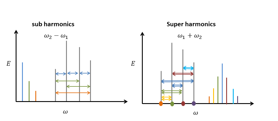
Fig. 16 Second order wave interaction for a given spectrum. The grey lines represent the primary waves and the coloured lines show the bound waves. The arrows indicate the interaction between two waves. The dots show the self-interaction of the primary waves.
Non-hydrostatic
Global continuity equation
As was outlined in the previous chapter the global continuity equation, which describes the relation between the free surface and the depth averaged discharge, is given by
A simple semi-discretisation of using central differences for the space derivative and using the Hansen scheme for the coupling between velocity and free surface results in
With \({}^{x} q_{i+{\tfrac{1}{2}} ,j}^{\*} = H_{i+{\tfrac{1}{2}} ,j}^{n} U_{i+{\tfrac{1}{2}} ,j}^{n+{\tfrac{1}{2}} }\),\({}^{y} q_{i,j+{\tfrac{1}{2}} }^{\*} =H_{i,j+{\tfrac{1}{2}} }^{n} V_{i,j+{\tfrac{1}{2}} }^{n+{\tfrac{1}{2}} }\) and the water depth is defined by a first order accurate upwind interpolation
The resulting scheme is only first order accurate by virtue of the upwind interpolations and mass conservative. When first order computations are considered accurate enough \(\eta_{i,j}^{n+1}\) is set to \(\eta_{i,j}^{n\*}\). For higher order accuracy the first order prediction is corrected using a limited version of the McCormack scheme. The corrector step reads
With \({}^{x} \Delta q_{i+{\tfrac{1}{2}} ,j}^{n\*} = U_{i+{\tfrac{1}{2}} ,j}^{n+{\tfrac{1}{2}} } \Delta H_{i+{\tfrac{1}{2}} ,j}\) and \(\Delta H_{i+{\tfrac{1}{2}} ,j}\) is given for positive flow as
Here \(\psi \left(r\right)\) denotes the minmod limiter. Similar expression can be constructed for negative flow. The expression for \({}^{y} \Delta q_{i,j+{\tfrac{1}{2}} }^{n\*}\) and \(\Delta H_{i,j+{\tfrac{1}{2}} }\) are obtained in a similar manner. Note that the total flux \({}^{x} q_{i+{\tfrac{1}{2}} ,j}^{n+{\tfrac{1}{2}} }\)at the cell boundaries thus reads
The predictor-corrector set is second order accurate in regions where the solution is smooth, and reduces locally to first order accuracy near discontinuities. Furthermore, the method remains mass conservative. Note that other flux limiters can be used instead of the minmod limiter. However, as the minmod limiter performed adequately, this has not been investigated. (for an overview of flux limiters see [Hirsch, 2007])
Local continuity equation
The depth averaged local continuity equation is given by
This equation is discretized using central differences
Missing grid variables\(\eta _{i+{\tfrac{1}{2}} ,j}^{n+1} ,\eta _{i,j+{\tfrac{1}{2}} }^{n+1}\) are approximated with upwind interpolation. Because there is no separate time evolution equation for the pressure the local continuity equation will be used to setup a discrete set of poison type equations in which the pressures are the only unknown quantities.
Horizontal Momentum
To obtain a conservative discretisation of the momentum equation the approach from [Stelling and Zijlema, 2003] is followed. However, to improve the accuracy of the method the combined space-time discretisation of the advection is done using a variant of the [MacCormack, 1969] is used. This scheme consists of a first order predictor step and a flux limited corrector step. The hydrostatic pressure is integrated using the midpoint rule and central differences, while the source terms and the turbulent stresses are integrated using an explicit Euler time integration. Formally the time integration is therefore first order accurate, but in regions where the turbulent stresses are negligible the scheme is of almost second order accuracy.
The depth averaged horizontal momentum equation for \(HU\)is given by
A first order accurate predictor step in time and space is then given as
Here Pr represents a discretisation of the dynamic pressure; T the effect of (turbulent) viscosity and S includes all other source terms. The discretisation of the (turbulent) viscous terms is given by central differences:
Here \(\bar{\bar{\nu }}_{i+{\tfrac{1}{2}} ,j+1}^{n+{\tfrac{1}{2}} }\) and \(\bar{\bar{H}}_{i+{\tfrac{1}{2}} ,j+1{\tfrac{1}{2}} }^{n+{\tfrac{1}{2}} }\) are obtained from the surrounding points by simple linear interpolation.
Due to the incompressible flow assumption the dynamic pressure does not have a separate time evolution equation, but instead it satisfies an elliptical equation in space. As such its effect cannot be calculated explicitly using values at the previous time level. However to improve the accuracy of the predictor step the effect of the dynamic pressure is included explicitly. To do this first the unknown pressure is decomposed as:
where the difference in pressure\(\Delta p_{i,j}^{n+1{\tfrac{1}{2}} }\) is generally small. In the predictor step the effect of the pressure is included explicitly using\(p_{i,j}^{n+{\tfrac{1}{2}} }\). In the corrector step the full Poisson equation is then solved for \(\Delta p_{i,j}^{n+1{\tfrac{1}{2}} }\). The pressure term in the predictor step is thus given as
Here \(\bar{p}_{i+1,j}^{n+{\tfrac{1}{2}} }\)represents the average pressure over the vertical which is approximated with\(\bar{p}_{i+1,j}^{n+{\tfrac{1}{2}} } ={\tfrac{1}{2}} p_{i+1,j}^{n+{\tfrac{1}{2}} }\), in which \(p_{i+1,j}^{n+{\tfrac{1}{2}} }\) is the pressure at the bottom. Furthermore \(p_{i+{\tfrac{1}{2}} ,j}^{n+{\tfrac{1}{2}} }\) is given as\(p_{i+{\tfrac{1}{2}} ,j}^{n+{\tfrac{1}{2}} } ={\tfrac{1}{2}} \left(p_{i+1,j}^{n+{\tfrac{1}{2}} } +p_{i,j}^{n+{\tfrac{1}{2}} } \right)\).
Currently is formulated with the depth integrated momentum as the primitive variable, and not the depth averaged velocity. To reformulate in terms of \(U\)we use the method by [Stelling and Zijlema, 2003]. First note that \(\left(HU\right)_{i+{\tfrac{1}{2}} ,j}^{n+{\tfrac{1}{2}} }\) and \(\left(HU\right)_{i+{\tfrac{1}{2}} ,j}^{\*}\) are approximated as \(\bar{H}_{i+{\tfrac{1}{2}} ,j}^{n} U_{i+{\tfrac{1}{2}} ,j}^{n+{\tfrac{1}{2}} }\) and \(\bar{H}_{i+{\tfrac{1}{2}} ,j}^{n+1} U_{i+{\tfrac{1}{2}} ,j}^{\*}\). Now using \(\left(HU\right)_{i+{\tfrac{1}{2}} ,j}^{n+{\tfrac{1}{2}} }\) is equivalent to:
Substituting into the full expressions (including those for \(V_{i,j+{\tfrac{1}{2}} }^{\*}\)) become:
Where we again use a first order upwind interpolation for \(U_{i+1,j}^{n+{\tfrac{1}{2}} }\)and\(U_{i,j+1}^{n+{\tfrac{1}{2}} }\). This is exactly the approximation used by [Stelling and Zijlema, 2003] and is fully momentum conservative.
The predictor step is first order accurate in both space and time due to the use of upwind approximations for and Euler explicit time integration for the advective terms, and first order time integration for the source/viscous terms. This level of accuracy is acceptable near shore, where strong non-linearity (wave breaking, flooding and drying) will force the use of small steps in space and time anyway. However, in the region where waves only slowly change (e.g. shoaling/refraction on mild slopes), the first order approximations suffer from significant numerical damping. To improve the accuracy of the numerical model in these regions a corrector step is implemented after the predictor step.
The corrector step is given by:
Or, when formulated in terms of the depth averaged velocity
The values of \(\Delta U_{i+1,j}^{n\*}\) are obtained from slope limited expressions. For positive flow these read:
Where \(\psi\) again denotes the minmod limiter. Similar expressions can be constructed for\(\Delta U_{i+{\tfrac{1}{2}} ,j+{\tfrac{1}{2}} }\),\(\Delta V_{i,j}\) and\(\Delta V_{i+{\tfrac{1}{2}} ,j+{\tfrac{1}{2}} }\).
The predictor-corrector set is second order accurate in regions where the solution is smooth, and reduces to first order accuracy near sharp gradients in the solutions to avoid unwanted oscillations. Furthermore, the method remains momentum conservative.
Vertical momentum equations
The vertical momentum equation is discretized in a similar manner to the horizontal momentum equations using the McCormack scheme. In terms of the depth averaged vertical velocity the predictor step is:
The pressures are defined on the cell faces and therefore do not have to be interpolated. Furthermore, we can exactly set the dynamic pressure at the free surface \(p_{i,j,1}^{n+{\tfrac{1}{2}} }\) to zero. The vertical velocities are defined on the cell faces and therefore the depth averaged velocity \(\bar{W}_{i,j}^{n+{\tfrac{1}{2}} }\) needs to be expressed in terms of the bottom and surface velocities. Using a simple central approximation gives
At the bottom the kinematic boundary condition is used for the vertical velocity:
Horizontal interpolation of \(\bar{W}_{i+{\tfrac{1}{2}} ,j}^{n+{\tfrac{1}{2}} }\) and \(\bar{W}_{i,j+{\tfrac{1}{2}} }^{n+{\tfrac{1}{2}} }\) is done using first order upwind similar to . The turbulent stresses are again approximated using a central scheme as
Thus combining, and explicit expressions for \(w_{i,j,1}^{\*}\) and \(w_{i,j,0}^{\*}\) are obtained.
The predicted values are again corrected using a variant of the McCormack scheme and including the pressure difference implicitly gives the corrector step:
Where \(\Delta \bar{W}_{i+{\tfrac{1}{2}} ,j}\) and \(\Delta \bar{W}_{i,j+{\tfrac{1}{2}} }\) are obtained using relations similar to . Note that similar to \(\bar{W}_{i,j}^{n+1{\tfrac{1}{2}} } ={\tfrac{1}{2}} \left(w_{i,j.1}^{n+1{\tfrac{1}{2}} } +w_{i,j,0}^{n+1{\tfrac{1}{2}} } \right)\)and again the kinematic boundary conditions is substituted for \(w_{i,j,0}^{n+1{\tfrac{1}{2}} }\).
The discrete vertical momentum balance of and looks very different from the relations found in [Zijlema and Stelling, 2005], [Zijlema and Stelling, 2008] and [Smit, 2008]. This is mainly due to the application of the McCormack scheme for the advection. The discretisation of the pressure term is numerically fully equivalent to either the Keller box scheme as used in [Zijlema and Stelling, 2005], [Zijlema and Stelling, 2008] or the Hermetian relation used in [Smit, 2008].
Advanced model coefficients
In General the main input parameters and files required by XBeach to start a simulation are explained. It explained how the user can switch on and off specific processes and how the user can define the model initial and boundary conditions. XBeach offers, however, many more parameters to fine-tune the simulation of different processes. These parameters are listed in the following subsections grouped by process. Most parameters are not relevant for the average XBeach user. Parameters marked with a plus (+) are considered advanced options that are recommended to stay untouched unless you know what you are doing.
Long and short wave boundary conditions
The parameters listed in the table below relate to boundary conditions for short waves (wave action balance model) and long waves (infragravity waves).
parameter |
description |
default |
range |
units |
|---|---|---|---|---|
nmax+ |
Maximum ratio of cg/c for computing long wave boundary conditions |
0.8 |
0.5 - 1.0 |
|
wbcevarreduce |
Reduction factor of short-wave group variance at the boundary |
1 |
0-1 |
|
bclwonly |
Switch to run boundary conditions with long waves only |
0 |
0 - 1 |
|
swkhmin |
Minimum kh value to include in wave action balance, lower included in nlswe |
-0.01 |
-0.01 - 0.35 |
|
wbcRemoveStokes |
Switch to remove long wave Stokes drift component at the offshore boundary |
1 |
0-1 |
|
wbcScaleEnergy |
Switch to correct random time series of wave height to exactly match input Hm0 |
0 |
0-1 |
|
cyclicdiradjust |
Adjust alongshore wave length to fit inside domain with cyclic boundary conditions |
0 |
0-1 |
Wave numerics
The parameters listed in the table below involve the numerical aspects of the wave action balance that solves the wave propagation in the model. The keyword scheme can be used to set the numerical scheme. To overcome the undesired effects of steepening of wave groups we implemented a correction to the second-order upwind scheme according to ([Beam and Warming, 1976]), which implies a small additional diffusion term which is a function of time step and group velocity. By default Warming and Beam (1976) is used.
parameter |
description |
default |
range |
units |
|---|---|---|---|---|
maxerror+ |
Maximum wave height error in wave stationary iteration |
0.0005 |
1e-05 - 0.001 |
m |
maxiter+ |
Maximum number of iterations in wave stationary |
500 |
2 - 1000 |
|
scheme+ |
Numerical scheme for wave propagation |
warmbeam |
upwind_1, lax_wendroff, upwind_2, warmbeam |
|
wavint |
Interval between wave module calls (only in stationary wave mode) |
600.0 |
1.0 - 3600.0 |
s |
Wave dissipation
The parameters listed in the table below involve the wave dissipation process. For instationary model runs use either break = roelvink1, roelvink2 or roelvink_daly. Note that the standard value gamma = 0.55 and n = 10 was calibrated for option break = roelvink1. For break = roelvink2 the wave dissipation is proportional to \({H}^{3}/h\) instead of \({H}^{2}\); this affects the calibration. For stationary runs the break = baldock option is suitable. The break = roelvink_daly option is a model in which waves start and stop breaking. Reducing gammax will reduce wave heights in very shallow water, probably 2 is a reasonable value.
parameter |
description |
default |
range |
units |
|---|---|---|---|---|
alpha+ |
Wave dissipation coefficient in roelvink formulation |
1.0 |
0.5 - 2.0 |
|
break |
Type of breaker formulation |
roelvink_daly |
roelvink1, baldock, roelvink2, roelvink_daly, janssen |
|
breakerdelay+ |
Switch to enable breaker delay model |
1.0 |
0.0 - 3.0 |
|
delta+ |
Fraction of wave height to add to water depth |
0.0 |
0.0 - 1.0 |
|
facrun |
Calibration coefficient for short wave runup |
1.0 |
0.0 - 2.0 |
|
facsd |
Fraction of the local wave length to use for shoaling delay depth |
1.0 |
0.0 - 2.0 |
|
fwcutoff |
Depth greater than which the bed friction factor is not applied |
1000.0 |
0.0 - 1000.0 |
|
gamma |
Breaker parameter in baldock or roelvink formulation |
0.46 |
0.4 - 0.9 |
|
gamma2 |
End of breaking parameter in roelvink daly formulation |
0.34 |
0.0 - 0.5 |
|
gammax+ |
Maximum ratio wave height to water depth |
2.0 |
0.4 - 5.0 |
|
n+ |
Power in roelvink dissipation model |
10.0 |
5.0 - 20.0 |
|
shoaldelay |
Switch to enable shoaling delay |
0 |
0 - 1 |
|
wavfriccoef |
Wave friction coefficient |
-123 |
||
wavfricfile |
Wave friction file |
<file> |
Rollers
The parameters listed in the table below involve the wave roller model. Using the roller model will give a shoreward shift in wave-induced setup, return flow and alongshore current. This shift becomes greater for lower beta values.
parameter |
description |
default |
range |
units |
|---|---|---|---|---|
beta+ |
Breaker slope coefficient in roller model |
0.08 |
0.05 - 0.3 |
|
rfb+ |
Switch to feed back maximum wave surface slope in roller energy balance, otherwise rfb = par%beta |
0 |
0 - 1 |
|
roller+ |
Switch to enable roller model |
1 |
0 - 1 |
Wave-current interaction
The parameters listed in the table below involve the process of wave-current interaction. With the switch wci one can turn off or on the wave-current interaction, the wave current interaction will result in a feedback of currents on the wave propagation. On top of that, hwci limits the computation of wave-current interaction in very shallow water where the procedure may not converge.
parameter |
description |
default |
range |
units |
|---|---|---|---|---|
cats+ |
Current averaging time scale for wci, in terms of mean wave periods |
4.0 |
1.0 - 50.0 |
Trep |
hwci+ |
Minimum depth until which wave-current interaction is used |
0.1 |
0.001 - 1.0 |
m |
hwcimax+ |
Maximum depth until which wave-current interaction is used |
100.0 |
0.01 - 100.0 |
m |
wci |
Turns on wave-current interaction |
0 |
0 - 1 |
Bed friction and viscosity
The parameters listed in the table below involve the settings for bed friction and viscosity influencing the flow in XBeach. The bed friction is influenced by the dimensionless friction coefficient cf or other formulation like the dimensional Chézy or Manning. The bed friction formulation applied needs to be determined with the keyword bedfriction. It is possible both to define one value (keyword: bedfriccoef) or to apply, spatially varying values for the bed friction. A spatial varying friction can be provided through an external file referenced via the keyword bedfricfile. The file has the same format as the bathymetry file explained in Grid and bathymetry.
The horizontal viscosity is composed of an overall background viscosity nuh and a viscosity depending on the roller dissipation tuned by nuhfac. In the alongshore direction the viscosity may be multiplied by a factor nuhv to account for additional advective mixing. It is also possible to use a user-defined value for the horizontal viscosity (keyword smag = 0)
parameter |
description |
default |
range |
units |
|---|---|---|---|---|
bedfriccoef |
Bed friction coefficient |
0.01 |
3.5e-05 - 0.9 |
|
bedfricfile |
Bed friction file (only valid with values of c) |
<file> |
||
bedfriction |
Bed friction formulation |
manning |
chezy, cf, white-colebrook, manning, white-colebrook-grainsize |
|
friction_acceleration |
Turn on or off the effect of acceleration on bed roughness (morrison) |
none |
none, mccall, nielsen |
|
friction_infiltration |
Turn on or off the effect of infiltration on bed roughness (conley and inman) |
0 |
0 - 1 |
|
friction_turbulence |
Turn on or off the effect of turbulence on bed roughness (reniers van thiel) |
0 |
0 - 1 |
|
gamma_turb |
Calibration factor for turbulence contribution to bed roughness |
1.0 |
0.0 - 2.0 |
|
nuh |
Horizontal background viscosity |
0.1 |
0.0 - 1.0 |
m^2s^-1 |
nuhfac+ |
Viscosity switch for roller induced turbulent horizontal viscosity |
0.0 |
0.0 - 1.0 |
|
nuhv |
Longshore viscosity enhancement factor, following svendsen (?) |
1.0 |
1.0 - 20.0 |
|
smag+ |
Switch for smagorinsky subgrid model for viscocity |
1 |
0 - 1 |
Flow numerics
The parameters listed in the table below involve the numerical aspects of the shallow water equations that solve the water motions in the model. Especially in very shallow water some processes need to be limited to avoid unrealistic behavior. For example hmin prevents very strong return flows or high concentrations and the eps determines whether points are dry or wet and can be taken quite small.
To prevent that the numerical limiter hmin is affected by the scale of the simulation the hmin is defined as
when oldhmin is 0 (default). This means that hmin is equal to the water depth (h) when the wave height (H) is smaller than the water depth. When the wave height is larger than the water depth, the hmin is equal to the water depth plus an additional contribution related to the wave height times the (deltahmin). if oldhmin is set to 1, the old implementation of hmin is applied, in which the minimum water depth for the retun flow computation is set to the value of hmin.
parameter |
description |
default |
range |
units |
|---|---|---|---|---|
eps |
Threshold water depth above which cells are considered wet |
0.005 |
0.001 - 0.1 |
m |
eps_sd |
Threshold velocity difference to determine conservation of energy head versus momentum |
0.5 |
0.0 - 1.0 |
m/s |
hmin |
Threshold water depth above which stokes drift is included |
0.0 |
0.001 - 1.0 |
m |
oldhu |
Switch to enable old hu calculation |
0 |
0 - 1 |
|
secorder+ |
Use second order corrections to advection/non-linear terms based on maccormack scheme |
0 |
0 - 1 |
|
umin |
Threshold velocity for upwind velocity detection and for vmag2 in equilibrium sediment concentration |
0.0 |
0.0 - 0.2 |
m/s |
deltahmin |
Dimensionless coefficent to determine the threshold water depth above which stokes drift is included |
0.1 |
0.0 - 1.0 |
|
oldhmin |
Switch to apply the old hmin parameter instead of the deltahmin |
0 |
0 - 1 |
Sediment transport
The parameters listed in the table below involve the process of sediment transport. The keywords facAs and facSk determine the effect of the wave form on the sediment transport, this is especially important in the nearshore. The facua is an alias setting in which both parameters can be varied at once. The wave form model itself is selected using the keyword waveform. Processes like short- and long-wave stirring and turbulence can be switched on or off using the keywords sws, lws and lwt. Several options for calibrating the sediment transport formulations are available as well as keywords to incorporate the bed slope effect.
parameter |
description |
default |
range |
units |
|---|---|---|---|---|
BRfac+ |
Calibration factor surface slope |
1.0 |
0.0 - 1.0 |
|
Tbfac+ |
Calibration factor for bore interval tbore: tbore = tbfac*tbore |
1.0 |
0.0 - 1.0 |
|
Tsmin+ |
Minimum adaptation time scale in advection diffusion equation sediment |
0.5 |
0.01 - 10.0 |
s |
bdslpeffdir |
Modify the direction of the sediment transport based on the bed slope |
none |
none, talmon |
|
bdslpeffdirfac |
Calibration factor in the modification of the direction |
1.0 |
0.0 - 2.0 |
|
bdslpeffini |
Modify the critical shields parameter based on the bed slope |
none |
none, total, bed |
|
bdslpeffmag |
Modify the magnitude of the sediment transport based on the bed slope, uses facsl |
roelvink_total |
none, roelvink_total, roelvink_bed, soulsby_total, soulsby_bed |
|
bed+ |
Calibration factor for bed transports |
1 |
0 - 1 |
|
bermslope |
Swash zone slope for (semi-) reflective beaches |
0.0 |
0.0 - 1.0 |
|
betad+ |
Dissipation parameter long wave breaking turbulence |
1.0 |
0.0 - 10.0 |
|
bulk+ |
Switch to compute bulk transport rather than bed and suspended load separately |
0 |
0 - 1 |
|
ci+ |
Mass coefficient in shields inertia term |
1.0 |
0.5 - 1.5 |
|
cm |
Mass coefficient in shields inertia term |
1.5 |
0.0 - 3.0 |
|
dilatancy |
Switch to reduce critical shields number due dilatancy |
0 |
0 - 1 |
|
facAs+ |
Calibration factor time averaged flows due to wave asymmetry |
0.2 |
0.0 - 1.0 |
|
facDc+ |
Option to control sediment diffusion coefficient |
1.0 |
0.0 - 1.0 |
|
facSk+ |
Calibration factor time averaged flows due to wave skewness |
0.15 |
0.0 - 1.0 |
|
facsl+ |
Factor bedslope effect |
1.6 |
0.0 - 1.6 |
|
facua+ |
Calibration factor time averaged flows due to wave skewness and asymmetry |
0.1 |
0.0 - 1.0 |
|
fallvelred |
Switch to reduce fall velocity for high concentrations |
0 |
0 - 1 |
|
form |
Equilibrium sediment concentration formulation |
vanthiel_vanrijn |
soulsby_vanrijn, vanthiel_vanrijn, vanrijn1993 |
|
jetfac |
Option to mimic turbulence production near revetments |
0.0 |
0.0 - 1.0 |
|
lws+ |
Switch to enable long wave stirring |
1 |
0 - 1 |
|
lwt+ |
Switch to enable long wave turbulence |
0 |
0 - 1 |
|
phit+ |
Phase lag angle in nielsen transport equation |
25.0 |
0.0 - 90.0 |
|
pormax |
Max porosity used in the experession of van rhee |
0.5 |
0.3 - 0.6 |
|
reposeangle |
Angle of internal friction |
30.0 |
0.0 - 45.0 |
deg |
rheeA |
A parameter in the van rhee expression |
0.75 |
0.75 - 2.0 |
|
smax+ |
Maximum shields parameter for equilibrium sediment concentration acc. diane foster |
-1.0 |
-1.0 - 3.0 |
|
sus+ |
Calibration factor for suspensions transports |
1 |
0 - 1 |
|
sws+ |
Switch to enable short wave and roller stirring and undertow |
1 |
0 - 1 |
|
tsfac+ |
Coefficient determining ts = tsfac * h/ws in sediment source term |
0.1 |
0.01 - 1.0 |
|
turb+ |
Switch to include short wave turbulence |
wave_averaged |
none, wave_averaged, bore_averaged |
|
turbadv+ |
Switch to activate turbulence advection model for short and or long wave turbulence |
none |
none, lagrangian, eulerian |
|
waveform |
Wave shape model |
vanthiel |
ruessink_vanrijn, vanthiel |
|
z0+ |
Zero flow velocity level in soulsby and van rijn (1997) sediment concentration |
0.006 |
0.0001 - 0.05 |
m |
Sediment transport numerics
The parameters listed in the table below involve the numerical aspects of sediment transport that are all considered advanced options. For example the maximum allowed sediment concentration can be varied with the keyword cmax. It is however not recommended varying these settings.
parameter |
description |
default |
range |
units |
|---|---|---|---|---|
cmax+ |
Maximum allowed sediment concentration |
0.1 |
0.0 - 1.0 |
|
sourcesink+ |
Switch to enable source-sink terms to calculate bed level change rather than suspended transport gradients |
0 |
0 - 1 |
|
thetanum+ |
Coefficient determining whether upwind (1) or central scheme (0.5) is used. |
1.0 |
0.5 - 1.0 |
|
dtlimts+ |
Factor of the timestep to determine the numerical limiter of the adaptation time. |
1.0 |
0 - 20.0 |
|
oldTsmin+ |
Switch to apply the tsmin parameter instead of the dtlimts.. |
0 |
0 - 1 |
Quasi-3D sediment transport
The parameters listed in the table below involve the tuning of quasi-3D sediment transport, if enabled. The most important setting is the kmax in which the user specifies the number of layers used in the quasi 3D sediment model.
parameter |
description |
default |
range |
units |
|---|---|---|---|---|
deltar |
Estimated ripple height |
0.025 |
0.001 - 1.0 |
|
kmax |
Number of sigma layers in quasi-3d model; kmax = 1 is without vertical structure of flow and suspensions |
100 |
1 - 1000 |
|
rwave |
User-defined wave roughness adjustment factor |
2.0 |
0.1 - 10.0 |
|
sigfac |
Dsig scales with log(sigfac) |
1.3 |
0.0 - 10.0 |
|
vicmol |
Molecular viscosity |
1e-06 |
0.0 - 0.001 |
|
vonkar |
Von karman constant |
0.4 |
0.01 - 1.0 |
Morphology
The parameters listed in the table below involve the morphological processes. The dryslp and wetslp keyword define the critical avalanching slope above and below water respectively. If the bed exceeds the relevant critical slope it collapses and slides downward (avalanching). To reduce the impact of these landslides the maximum bed level change due to avalanching is limited by the nTrepAvaltime parameter.
The keyword morfac enables the user to decouple the hydrodynamical and the morphological time. This is suitable for situations where the morphological process is much slower than the hydrodynamic process. The factor defined by the morfac keyword is applied to all morphological change. A morfac = 10 therefore results in 10 times more erosion and deposition in a given time step than usual. The simulation time is however then shortened with the same factor to obtain an approximate result more quickly. The user can prevent the simulation time to be adapted to the morfac value by setting morfacopt to zero. The keywords morstart and morstop let the user enable the morphological processes in XBeach only for a particular period during the (hydrodynamic) simulation. These options can be useful if a spin-up time is needed for the hydrodynamics.
The struct and ne_layer keywords enable the user to specify non-erodible structures in the model. To switch on non-erodible structures use struct = 1. The location of the structures is specified in an external file referenced by the ne_layer keyword. The file has the same format as the bathymetry file explained in Grid and bathymetry. The values of the file define the thickness of the erodible layer on top of the non-erodible layer. A ne_layer file with only zeros therefore defines a fully non-erodible bathymetry and a file with only tens means a erodible layer of 10 meters. Only at the grid cells where the value in the ne_layer file is larger than zero erosion can occur. Non-erodible layers are infinitely deep and thus no erosion underneath these layers can occur.
parameter |
description |
default |
range |
units |
|---|---|---|---|---|
dryslp |
Critical avalanching slope above water (dz/dx and dz/dy) |
1.0 |
0.1 - 2.0 |
|
dzmax+ |
Maximum bed level change due to avalanching |
0.05 |
0.0 - 1.0 |
m/s/m |
hswitch+ |
Water depth at which is switched from wetslp to dryslp |
0.1 |
0.01 - 1.0 |
m |
lsgrad |
Factor to include longshore transport gradient in 1d simulationsdsy/dy=lsgrad*sy; dimension 1/length scale of longshore gradients |
0.0 |
-0.1 - 0.1 |
1/m |
morfac |
Morphological acceleration factor |
1.0 |
0.0 - 1000.0 |
|
morfacopt+ |
Switch to adjusting output times for morfac |
1 |
0 - 1 |
|
morstart |
Start time morphology, in morphological time |
0.0 |
0.0 - par%tstop |
s |
morstop |
Stop time morphology, in morphological time |
2000.0 |
0.0 - 10000000.0 |
s |
ne_layer |
Name of file containing thickness of the erodible layer |
<file> |
||
struct |
Switch for enabling hard structures |
0 |
0 - 1 |
|
wetslp |
Critical avalanching slope under water (dz/dx and dz/dy) |
0.3 |
0.1 - 1.0 |
Bed update
The parameters listed in the table below involve the settings for the bed update process especially in the case multiple sediment fractions and bed layers are involved. The frac_dz, split and merge keywords determine the fraction of the variable bed layer thickness at which the layer is split or merged respectively with the surrounding bottom layers. The variable layer is chosen using the nd_var keyword.
Pre-defined bed evolution can be used with the keywords setbathy that is used to turn user-imposed bed level change on, nsetbathy that determines the number of imposed bed level conditions and setbathyfile that references a file that specifies the time series of imposed bed levels. If the setbathy option is used, XBeach will automatically interpolate the bed level at each computational time step from the imposed bed level time series.
The setbathyfile file must contain a time series (of length nsetbathy) of the bed level at every grid point in the XBeach model. The format of the setbathyfile file is such that each imposed bed level starts with the time at which the bed level should be applied (in seconds relative to the start of the simulation), followed on a new line by the bed level in each grid cell in an identical manner to the normal initial bathymetry file (e.g., one line per transect in the x-direction). The following imposed bed level condition starts on a new line with the time at which the condition is imposed and the bed levels at that time, etc. An example of a setbathyfile is given below.
setbathyfile.dep (generalized)
<t 0>
<z 1,1> <z 2,1> <z 3,1> ... <z nx,1> <z nx+1,1>
<z 1,2> <z 2,2> <z 3,2> ... <z nx,2> <z nx+1,2>
<z 1,3> <z 2,3> <z 3,3> ... <z nx,3> <z nx+1,3>

...

<z 1,ny> <z 2,ny> <z 3,ny> ... <z nx,ny> <z nx+1,ny>
<z 1,ny+1> <z 2,ny+1> <z 3,ny+1> ... <z nx,ny+1> <z nx+1,ny+1>
<t 1>
<z 1,1> <z 2,1> <z 3,1> ... <z nx,1> <z nx+1,1>
<z 1,2> <z 2,2> <z 3,2> ... <z nx,2> <z nx+1,2>
<z 1,3> <z 2,3> <z 3,3> ... <z nx,3> <z nx+1,3>

...

<z 1,ny> <z 2,ny> <z 3,ny> ... <z nx,ny> <z nx+1,ny>
<z 1,ny+1> <z 2,ny+1> <z 3,ny+1> ... <z nx,ny+1> <z nx+1,ny+1>

...

...

<t nsetbathy>
<z 1,1> <z 2,1> <z 3,1> ... <z nx,1> <z nx+1,1>
<z 1,2> <z 2,2> <z 3,2> ... <z nx,2> <z nx+1,2>
<z 1,3> <z 2,3> <z 3,3> ... <z nx,3> <z nx+1,3>

...

<z 1,ny> <z 2,ny> <z 3,ny> ... <z nx,ny> <z nx+1,ny>
<z 1,ny+1> <z 2,ny+1> <z 3,ny+1> ... <z nx,ny+1> <z nx+1,ny+1>
setbathyfile.dep (short 1D example, nx = 20, ny = 0, nsetbathy = 4)
0    -20 -18 -16 -14 -12 -10 -8 -6 -5 -4 -3   -2   -1    -0.5  0    0.5 1   2   3   4   5
1200 -20 -18 -16 -14 -12 -10 -8 -6 -5 -4 -3   -1.8 -0.75 -0.25 0    0.2 0.7 2   3   4   5
2400 -20 -18 -16 -14 -12 -10 -8 -6 -5 -4 -2.5 -1.6 -0.5  -0.3  0    0.1 0.6 1.5 3   4   5
3600 -20 -18 -16 -14 -12 -10 -8 -6 -5 -4 -2   -1.4 -0.3   0    0.05 0.1 0.6 1   2.2 3.5 5
Note that if the setbathy option is used, the initial bed level is derived from an interpolation of the setbathyfile file time series, not from the depfile file. It is strongly advised to turn of the computation of morphological updating (keyword: morphology = 0) if the setbathy option is used, as the computed morphological change will be overridden by the imposed morphological change.
parameter |
description |
default |
range |
units |
|---|---|---|---|---|
frac_dz+ |
Relative thickness to split time step for bed updating |
0.7 |
0.5 - 0.98 |
|
merge+ |
Merge threshold for variable sediment layer (ratio to nominal thickness) |
0.01 |
0.005 - 0.1 |
|
nd_var+ |
Index of layer with variable thickness |
2 |
1 - par%nd |
|
nsetbathy+ |
Number of prescribed bed updates |
1 |
1 - 1000 |
|
setbathyfile+* |
Name of prescribed bed update file |
<file> |
||
split+ |
Split threshold for variable sediment layer (ratio to nominal thickness) |
1.01 |
1.005 - 1.1 |
Groundwater flow
The parameters listed in the table below involve the process of groundwater flow. The vertical permeability coefficient in the vertical can be set differently than that of the horizontal using the keywords kz and kz respectively. The initial bed level of the aquifer is read from an external file referenced by the aquiferbotfile keyword and the initial groundwater head can be set to either a uniform value using the gw0 keyword or to spatially varying values using an external file referenced by the gw0file keyword. Both files have the same format as the bathymetry file explained in Grid and bathymetry.
parameter |
description |
default |
range |
units |
|---|---|---|---|---|
aquiferbot+ |
Level of uniform aquifer bottom |
-10.0 |
-100.0 - 100.0 |
m |
aquiferbotfile+ |
Name of the aquifer bottom file |
<file> |
||
dwetlayer+ |
Thickness of the top soil layer interacting more freely with the surface water |
0.1 |
0.01 - 1.0 |
m |
gw0+ |
Level initial groundwater level |
0.0 |
-5.0 - 5.0 |
m |
gw0file+ |
Name of initial groundwater level file |
<file> |
||
gwReturb+ |
Reynolds number for start of turbulent flow in case of gwscheme = turbulent |
100.0 |
1.0 - 600.0 |
|
gwfastsolve |
Reduce full 2d non-hydrostatic solution to quasi-explicit in longshore direction |
0 |
0 - 1 |
|
gwheadmodel+ |
Model to use for vertical groundwater head |
parabolic |
parabolic, exponential |
|
gwhorinfil+ |
Switch to include horizontal infiltration from surface water to groundwater |
0 |
0 - 1 |
|
gwnonh+ |
Switch to turn on or off non-hydrostatic pressure for groundwater |
0 |
0 - 1 |
|
gwscheme+ |
Scheme for momentum equation |
laminar |
laminar, turbulent |
|
kx+ |
Darcy-flow permeability coefficient in x-direction |
0.0001 |
1e-05 - 0.1 |
ms^-1 |
ky+ |
Darcy-flow permeability coefficient in y-direction |
0.0001 |
1e-05 - 0.1 |
ms^-1 |
kz+ |
Darcy-flow permeability coefficient in z-direction |
0.0001 |
1e-05 - 0.1 |
ms^-1 |
Non-hydrostatic correction
The parameters listed in the table below involve the settings for the non-hydrostatic option (keyword: wavemodel = nonh). These are all considered advanced options and it is thus recommended not to change these
parameter |
description |
default |
range |
units |
|---|---|---|---|---|
Topt+ |
Absolute period to optimize coefficient |
10.0 |
1.0 - 20.0 |
s |
breakviscfac+ |
Factor to increase viscosity during breaking |
1.5 |
1.0 - 3.0 |
|
breakvisclen+ |
Ratio between local depth and length scale in extra breaking viscosity |
1.0 |
0.75 - 3.0 |
|
dispc+ |
Coefficient in front of the vertical pressure gradient |
-1.0 |
0.1 - 2.0 |
? |
kdmin+ |
Minimum value of kd (pi/dx > min(kd)) |
0.0 |
0.0 - 0.05 |
|
maxbrsteep+ |
Maximum wave steepness criterium |
0.4 |
0.3 - 0.8 |
|
nhbreaker+ |
Non-hydrostatic breaker model |
2 |
0 - 2 |
|
nhlay+ |
Layer distribution in the nonhydrostatic model, default = 0.33 |
0.33 |
0.0 - 1.0 |
|
nonhq3d |
Turn on or off the the reduced two-layer nonhydrostatic model, default = 0 |
0 |
0 - 1 |
|
reformsteep+ |
Wave steepness criterium to reform after breaking |
0.25d0*par%maxbrsteep |
0.0 - 0.95d0*par%maxbrsteep |
|
secbrsteep+ |
Secondary maximum wave steepness criterium |
0.5d0*par%maxbrsteep |
0.0 - 0.95d0*par%maxbrsteep |
|
solver+ |
Solver used to solve the linear system |
tridiag |
sip, tridiag |
|
solver_acc+ |
Accuracy with respect to the right-hand side usedin the following termination criterion: ||b-ax || < acc*||b|| |
0.005 |
1e-05 - 0.1 |
|
solver_maxit+ |
Maximum number of iterations in the linear sip solver |
30 |
1 - 1000 |
|
solver_urelax+ |
Underrelaxation parameter |
0.92 |
0.5 - 0.99 |
Physical constants
The parameters listed in the table below involve physical constants used by XBeach. The gravitational acceleration and density of water are universally used coefficient. The depthscale is a factor in order to set different cut-off values like eps and hswitch. A value of the depthscale lower than one means the cut-off values will increase.
parameter |
description |
default |
range |
units |
|---|---|---|---|---|
depthscale+ |
Depthscale of (lab)test simulated, affects eps, hmin, hswitch and dzmax |
1.0 |
1.0 - 200.0 |
|
g |
Gravitational acceleration |
9.81 |
9.7 - 9.9 |
ms^-2 |
rho |
Density of water |
1025.0 |
1000.0 - 1040.0 |
kgm^-3 |
Coriolis force
The parameters listed in the table below involve the settings for incorporating the effect of Coriolis on the shallow water equations. The keywords are universally used coefficients.
parameter |
description |
default |
range |
units |
|---|---|---|---|---|
lat+ |
Latitude at model location for computing coriolis |
0.0 |
-90.0 - 90.0 |
deg |
wearth+ |
Angular velocity of earth calculated as: 1/rotation_time (in hours) |
1.d0/24.d0 |
0.0 - 1.0 |
hour^-1 |
MPI
The parameters listed in the table below involve the settings for parallelization of XBeach. When running XBeach in parallel mode, the model domain is subdivided in sub models and each sub model is then computed on a separate core. This will increase the computational speed of the model. The sub models only exchange information over their boundaries when necessary. The MPI parameters determine how the model domain is subdivided. The keyword mpiboundary can be set to auto, x, y or man. In auto mode the model domain is subdivided such that the internal boundary is smallest. In x or y mode the model domain is subdivided in sub models extending to either the full alongshore or the full cross-shore extent of the model domain. In man mode the model domain is manually subdivided using the values specified with the mmpi and nmpi keywords. The number of sub models is not determined by XBeach itself, but by the MPI wrapper (e.g. MPICH2 or OpenMPI).
parameter |
description |
default |
range |
units |
|---|---|---|---|---|
mmpi+ |
Number of domains in cross-shore direction when manually specifying mpi domains |
2 |
1 - 100 |
|
mpiboundary+ |
Fix mpi boundaries along y-lines, x-lines, use manual defined domains or find shortest boundary automatically |
auto |
auto, x, y, man |
|
nmpi+ |
Number of domains in alongshore direction when manually specifying mpi domains |
4 |
1 - 100 |
Output projection
The parameters listed in the table below involve the projection of the model output. These settings do not influence the model results in anyway. The rotate keyword can be used to rotate the model output with an angle specified by the keyword alfa. The projection string can hold a string specifying the coordinate reference system used and is stored in the netCDF output file as metadata.
parameter |
description |
default |
range |
units |
|---|---|---|---|---|
projection+ |
Projection string |
|||
remdryoutput |
Remove dry output points from output data of zs etc. |
1 |
0 - 1 |
|
rotate |
Rotate output as postprocessing with given angle |
1 |
0 - 1 |